Announcing mpmath 0.15

June 6, 2010

I’m happy to announce the release of mpmath 0.15!

This should’ve happened earlier, but I was obstructed by other obligations (in particular, finishing my master’s thesis). The good news is that I will be working full-time on special functions in mpmath and Sage again this summer thanks to sponsorship provided by William Stein (with money from an NSF grant). I will also come to Sage Days 23 (July 5-9, Leiden, the Netherlands) and Sage Days 24 (July 17-22, Linz, Austria) which should be as fun as SD15.

What’s new in mpmath 0.15? As usual, the details can be found in the CHANGES file and the list of commits. Most major changes were covered in detail in previous blog posts, so I will first of all simply link to those posts along with short summaries:

Speedups of elementary functions - cos, sin, atan, cosh, sinh, exp and all derived functions are now faster. Of particular note, trigonometric functions use an asymptotically faster algorithm (all elementary functions have similar asymptotic performance now).

A new gamma function implementation - the gamma function and log-gamma functions have been rewritten scratch, using faster algorithms and code optimizations. The new versions are uniformly faster than the old ones, and tens or hundreds of times faster in many important situations. They are also more accurate in some special cases (near singularities, for complex arguments with extremely small real part, …).

Numerical multidimensional infinite series - nsum() can now evaluate series (finite or infinite) in any number of dimensions

Computing large zeta zeros with mpmath - Juan Arias de Reyna has implemented code for computing the nth zero of the Riemann zeta function on the critical line for arbitrarily large n. On a related note, the Riemann zeta function code has been optimized (mostly through elimination of low-level overhead) to speed up such computations.

Hypergeneralization - generalized 2D hypergeometric series, bilateral hypergeometric series and some q-analogs (q-Pochhammer symbol, q-factorial, q-gamma function, q-hypergeometric series) have been implemented.

In addition, there are many changes that I haven’t had time to blog about yet. I will now write briefly about some of these:

Elliptic functions

The support for working with elliptic functions has been improved. Instead of just the standard three, all 12 Jacobi elliptic functions are now available via ellipfun, e.g. the cd-function:

>>> from mpmath import *
>>> mp.dps = 25; mp.pretty = True
>>> ellipfun('cd', 3.5, 0.5)
-0.9891101840595543931308394
>>> cd = ellipfun('cd')
>>> cd(3.5, 0.5)
-0.9891101840595543931308394

Functions qfrom(), qbarfrom(), mfrom(), kfrom(), taufrom() have also been added to convert between the various forms of arguments to elliptic functions (nomes (two definitions), parameters, moduli, half-period ratios). If you’re like me and never can remember such formulas, let alone avoid messing up when trying to apply them, this can be quite convenient. Some functions (in particular, ellipfun also support direct choice of convention using keyword arguments):

>>> ellipfun('sn',2,1+1j)    # default is m
(1.333680690847080418060154 - 0.2084318767795699518406447j)
>>> ellipfun('sn',2,q=qfrom(m=1+1j))
(1.333680690847080418060154 - 0.2084318767795699518406447j)
>>> ellipfun('sn',2,k=kfrom(m=1+1j))
(1.333680690847080418060154 - 0.2084318767795699518406447j)
>>> ellipfun('sn',2,tau=taufrom(m=1+1j))
(1.333680690847080418060154 - 0.2084318767795699518406447j)

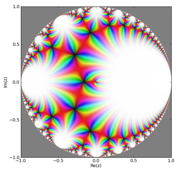
Another new function is the Klein j-invariant (or rather, the “absolute invariant” or “J-function” which differs by a constant factor, and also is the normalization used by Mathematica). A nice application is to compute the Laurent series expansion in terms of the (number-theoretic) nome, giving a famous integer sequence:

>>> mp.dps = 15
>>> taylor(lambda q: 1728*q*kleinj(qbar=q), 0, 5, singular=True)
[1.0, 744.0, 196884.0, 21493760.0, 864299970.0, 20245856256.0]

The J-function also looks pretty when plotted, here as a function of the number-theoretic nome within the unit circle:

fp.cplot(lambda q: fp.kleinj(qbar=q), [-1,1], [-1,1], points=400000)

As a function of the half-period ratio τ, defined in the upper half-plane:

fp.cplot(lambda t: fp.kleinj(tau=t), [-1,2], [0,1.5], points=100000)

Complex interval arithmetic

The support for interval arithmetic has been extended; there is also a new interface for intervals. It is no longer possible to call mpmath.exp etc. directly with interval arguments; instead all interval arithmetic has been moved to a separate context object called iv (similar to the separate interface for working with Python float/complex in mpmath). For example:

>>> iv.dps = 5; iv.pretty = True
>>> iv.mpf(1)/3
[0.3333330154, 0.3333334923]
>>> iv.sin(1)
[0.8414707184, 0.8414716721]
>>> iv.sin([1,2])
[0.8414707184, 1.0]
>>> iv.sin([1,3])
[0.141119957, 1.0]

The interface change was done to simplify the implementation; separating out interval arithmetic also helps avoid inadvertent mixing of interval and non-interval arithmetic.

There is also some support for complex interval arithmetic, including some elementary functions (exp, log, cos, sin, power).

>>> iv.mpc('1.3','1.4') ** 2
([-0.2700066566, -0.2699956894] + [3.639995575, 3.640010834]*j)
>>> iv.mpc('1.3','1.4') ** iv.mpc('1.2','-0.7')
([3.329280853, 3.329311371] + [1.967472076, 1.967498779]*j)
>>> iv.dps = 25
>>> iv.mpc('1.3','1.4') ** 2
([-0.270000000000000000000000061005, -0.269999999999999999999999912371] +
[3.63999999999999999999999988419, 3.64000000000000000000000009099]*j)
>>> mp.cos(2+3j)
(-4.189625690968807230132555 - 9.109227893755336597979197j)
>>> iv.cos(2+3j)
([-4.18962569096880723013255508975, -4.18962569096880723013255498635] + 
[-9.1092278937553365979791973006, -9.10922789375533659797919709381]*j)

Verifying Euler’s identity:

>>> iv.dps = 5
>>> iv.exp(1j * iv.pi)
([-1.0, -0.9999990463] + [-1.279517164e-6, 2.535183739e-6]*j)
>>> iv.dps = 25
>>> iv.exp(1j * iv.pi)
([-1.0, -0.999999999999999999999999987075] +
[-1.8806274411915714063022730148e-26, 3.28925138726485156164403137746e-26]*j)

Rigorous complex linear algebra:

>>> iv.dps = 15
>>> A = iv.matrix([[2,-2,1],[1,0,2],[1,1,2]])
>>> b = iv.matrix([1,2+2j,5])
>>> iv.lu_solve(A,b)
[ ([4.0, 4.0] + [-3.3333333333333333339, -3.333333333333333333]*j)]
[([3.0, 3.0] + [-2.0000000000000000004, -1.9999999999999999998]*j)]
[ ([-1.0, -1.0] + [2.6666666666666666665, 2.666666666666666667]*j)]
>>> A*iv.lu_solve(A,b)
[([1.0, 1.0] + [-8.8817841970012523234e-16, 1.7763568394002504647e-15]*j)]
[         ([2.0, 2.0] + [1.9999999999999995559, 2.0000000000000008882]*j)]
[([5.0, 5.0] + [-8.8817841970012523234e-16, 1.7763568394002504647e-15]*j)]

Partial derivatives

This is rather simple, but very convenient. diff can now compute partial derivatives of arbitrary order for multivariable functions. For example, a first derivative with respect to the second argument:

>>> diff(lambda x,y: 3*x*y + 2*y - x, (0.25, 0.5), (0,1))
2.75

The first derivative with respect to both x and y:

>>> diff(lambda x,y: 3*x*y + 2*y - x, (0.25, 0.5), (1,1))
3.0

Second derivative with respect to a parameter of a hypergeometric function ₂F₁(a,b,c,z); tenth derivative with respect to the argument; first derivative with respect to two parameters and fourth derivative with respect to the argument:

>>> diff(hyp2f1, (1,2,3,0.5), (0,0,2,0))
0.2306514802159766624657329
>>> diff(hyp2f1, (1,2,3,0.5), (0,0,0,10))
672869392.1810426015397572
>>> diff(hyp2f1, (1,2,3,0.5), (1,0,1,4))
-585.1335939248098118753126

That’s it for now. Stay tuned for many new features in the near future!

fredrikj.net | Blog index | RSS feed | Follow me on Mastodon | Become a sponsor