Incomplete elliptic integrals complete

June 21, 2010

I’m very happy to finally have implemented incomplete elliptic integrals in mpmath (they were probably the most-requested missing special functions). Now mpmath can compute the three classical (Legendre) elliptic integrals F(φ, m), E(φ, m), Π(n, φ, m) as well Carlson’s symmetric integrals R_F, R_C, R_J, R_D, R_G. Previously only the complete integrals K(m) and E(m) were available.

The functions are called, respectively, ellipf, ellipe, ellippi, elliprf, elliprc, elliprj, elliprd, elliprg, although this could change before the release. For the code, see r1162, r1166 and adjacent commits; documentation is available in the elliptic functions section.

This work was possible thanks to the support of NSF grant DMS-0757627, gratefully acknowledged.

Elliptic integral basics

What are elliptic integrals and why are they important? As the name suggests, they are related to ellipses. Given an ellipse of width 2a and height 2b, i.e. satisfying

or using an angular coordinate θ

the arc length along the ellipse from θ = 0 to θ = φ is given by

where m = 1-(a/b)^2 is the so-called elliptic parameter.

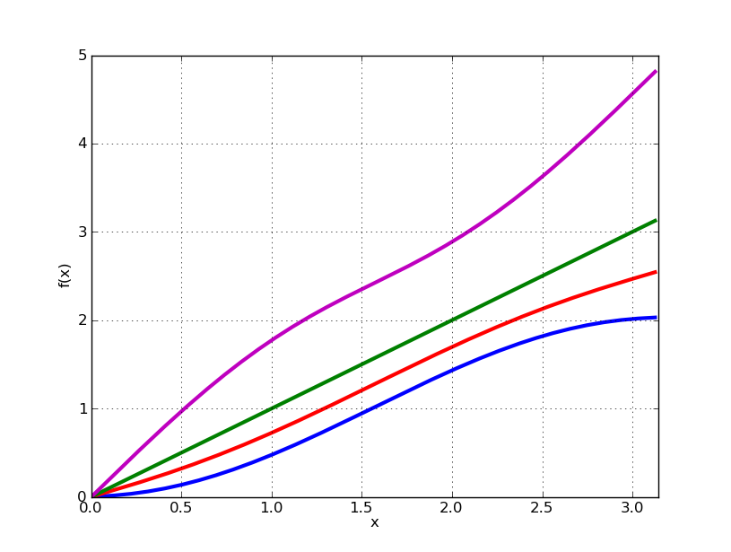
Here are some plots of half-ellipses of various proportions, and the corresponding arc lengths:

a = 1
b1 = 0.1; f1 = lambda x: b1*sqrt(1 - (x/a)**2)
b2 = 0.6; f2 = lambda x: b2*sqrt(1 - (x/a)**2)
b3 = 1.0; f3 = lambda x: b3*sqrt(1 - (x/a)**2)
b4 = 2.0; f4 = lambda x: b4*sqrt(1 - (x/a)**2)
plot([f1,f2,f3,f4], [-1,1])
g1 = lambda phi: b1*ellipe(phi, 1-(a/b1)**2)
g2 = lambda phi: b2*ellipe(phi, 1-(a/b2)**2)
g3 = lambda phi: b3*ellipe(phi, 1-(a/b3)**2)
g4 = lambda phi: b4*ellipe(phi, 1-(a/b4)**2)
plot([g1,g2,g3,g4], [0,pi])

The preceding formulas are sometimes seen with a and b switched, which simply corresponds to transposing x and y as the reference axis (above, the integration is assumed to start on the x axis). One can readily confirm that E(φ, m) satisfies obvious geometric symmetries:

>>> a = 0.5
>>> b = 0.25
>>> m1 = 1-(a/b)**2
>>> m2 = 1-(b/a)**2
>>> b*ellipe(pi/2,m1)           # Arc length of quarter-ellipse
0.6055280137842297624017815
>>> a*ellipe(pi/2,m2)
0.6055280137842297624017815
>>> a*ellipe(pi/4,m2) + b*ellipe(pi/4,m1)
0.6055280137842297624017815
>>> a*ellipe(pi/3,m2) + b*ellipe(pi/6,m1)
0.6055280137842297624017815

Elliptic integrals have countless uses in geometry and physics, and even in pure mathematics. They are related to Jacobi elliptic functions (already available in mpmath), which essentially are inverse functions of elliptic integrals:

>>> m = 0.5
>>> sn = ellipfun('sn')
>>> ellipf(asin(sn('0.65', m)), m)
0.65

More information about elliptic integrals can be found in DLMF Chapter 19.

Implementation

Implementing incomplete elliptic integrals properly is fairly complicated. When people have asked for them in the past, I just suggested using numerical integration. This works quite well most of the time, but it’s inefficient (and possibly gives poor accuracy) at high precision, for large arguments, or near singularities. Another approach — computing incomplete integrals from Appell hypergeometric functions (available in mpmath) — basically has the same drawbacks.

The numerically conscious way to compute elliptic integrals is to firstly exploit symmetries to obtain a small standard domain, and then using transformation formulas to reduce the magnitude of the arguments until the first few terms of the hypergeometric series give full accuracy (the arithmetic-geometric mean for the complete integrals, which leads to some of the fastest ways to compute π, is a special case of this process).

The transformations for Legendre’s integrals are known as Landen’s transformations. A more modern alternative, that I’ve chosen to use, is to represent Legendre’s integrals in terms of Carlson’s symmetric integrals which have much simpler structure. Although Carlson’s integrals are mainly intended for internal use, I’ve exposed them as top-level functions since it wasn’t much extra work and some users may well find them useful. (Carlson’s forms seem to become increasingly standard.)

Carlson’s paper is very readable and provides almost complete descriptions of the algorithms, including error bounds, which helped my implementation work tremendously. The error bounds are not rigorous in all cases, but good enough most of the time. Unfortunately, there are many special cases to consider, and Carlson does not address all of them explicitly, so putting it all together nevertheless involved a bit of work (and there are still some minor issues to fix).

Complex branch structure

One major issue is how to define the elliptic integrals for complex (or in some places, negative) parameters. Because the integrands defining Legendre’s elliptic integrals involve square roots of periodic functions, they have very complicated branch structure. I have chosen the periodic extension of the branches resulting naturally from use of the Carlson forms on -π/2 < Re(z) < π/2. I believe this is equivalent to choosing the principal-branch square root in the integrand and integrating along a path where the principal branch is continuous.

For example, consider E(φ, 3+4i). The integrand (with the principal square root, as computed by sqrt) and the elliptic integral computed by ellipe are plotted below:

>>> cplot(lambda z: sqrt(1-(3+4j)*sin(z)**2), points=50000)

>>> cplot(lambda z: ellipe(z, 3+4j), points=50000)

It can be seen that the cuts have the same shape in both images (the branch points are necessarily the same). As the following figure shows, if we are to integrate from z = 0 to z = -2+4i (X), a straight path (black) will be bad as it crosses a branch cut (O). However, the modified path (blue) avoiding the branch cut by passing through z = -2 is fine:

We can confirm this with numerical integration:

>>> ellipe(-2+4j, 3+4j)
(36.45544164923053561755261 + 49.28080768743760310823023j)
>>> quad(lambda z: sqrt(1-(3+4j)*sin(z)**2), [0,-2+4j])
(19.65109997738606076596704 + 46.63216059660102110020723j)
>>> quad(lambda z: sqrt(1-(3+4j)*sin(z)**2), [0,-2,-2+4j])
(36.45544164923053561755261 + 49.28080768743760310823023j)

Unfortunately, Mathematica doesn’t use quite the same branch cuts for its elliptic integrals. I don’t have Mathematica available to create a plot for comparison purposes, but I think it basically uses vertical cuts instead of the curvilinear cuts seen in the images above. There are probably good reasons for doing this, presumably that it simplifies symbolic definite integration, although it seems to complicate the evaluation and formulaic representation of the functions. It would perhaps be good to support both conventions.

As far as the symmetric functions are concerned, they have the nice property that although they involve non-principal square roots (chosen so as to be continuous along the real line), Carlson’s algorithm gives the continuous branch automatically. For example, if we consider the first function

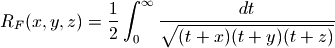
with x = i-1, y = i, z = 0, then as the following plot shows, the principal branch of the integrand has a discontinuity at t = 1/2:

>>> x,y,z = j-1,j,0
>>> f = lambda t: 1/sqrt((t+x)*(t+y)*(t+z))
>>> plot(f, [0,3])

To obtain the correct integrand, we switch to the negative square root on the left of the discontinuity (the positive sign should be used on the right because, for continuity with real parameters, we want the principal square root as t → +∞):

>>> g = lambda t: f(t) if t >= 0.5 else -f(t)
>>> plot(g, [0,3])

A quick test shows that f is wrong and g is right:

>>> extradps(25)(quad)(f, [0,inf])/2
(1.110136183412179775397387 - 0.04278194644898641314159222j)
>>> extradps(25)(quad)(g, [0,inf])/2
(0.7961258658423391329305694 - 1.213856669836495986430094j)
>>> elliprf(x,y,z)
(0.7961258658423391329305694 - 1.213856669836495986430094j)

In summary, branch cuts of special functions are a tricky business, and standards don’t always exist, so both developers and users need to be careful working with them.

fredrikj.net | Blog index | RSS feed | Follow me on Mastodon | Become a sponsor