Euler-Maclaurin summation of hypergeometric series

July 28, 2010

I recently fixed another corner case (it’s always the corner cases that are hard!) in the hypergeometric function evaluation code in mpmath.

The difficulty in question concerns the functions _pF_p-1(…; …; z), of which the Gauss hypergeometric function ₂F₁ is an important special case. These functions can be thought of as generalizations of the geometric series

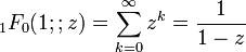
and the natural logarithm

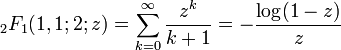
and share the property that the hypergeometric (Maclaurin) series has radius of convergence 1, with a singularity (either algebraic or logarithmic, as above) at z = 1.

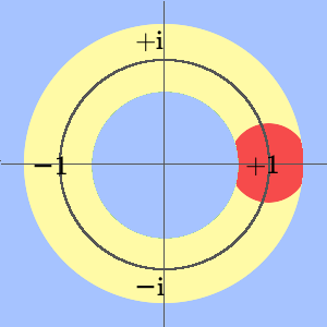
Numerical evaluation is fairly easy for z in most of the complex plane. The series for _pF_p-1(…; …; z) converges like the geometric series, so direct summation works well for, say, |z| ≤ r 0.9. Likewise, there is an analytic continuation formula which transforms z to 1/z, allowing evaluation for (say) |z| ≥ 1.1.

The remaining shell around the unit circle 0.9 < |z| < 1.1 is the difficult region. In fact, ₂F₁ can still (essentially) be computed using exact transformations here, but the higher cases remain difficult. As mentioned in an earlier post, mpmath handles this by calling nsum() which applies convergence acceleration to the slowly converging series. In particular, nsum implements the (generalized) Shanks transformation which is extremely efficient for this particular type of series – in fact, it works outside the radius of convergence (Shanks transformation effectively computes a Padé approximant), so it can be used anywhere in the difficult shell.

Still, the Shanks transformation is most efficient when arg(z) = ±π and unfortunately degenerates as arg(z) → 0, i.e. close to z = 1. nsum also implements Richardson extrapolation, which sometimes works at z = 1, but only for special parameter combinations in the hypergeometric series (although those special combinations happen to be quite important – they include the case where the hypergeometric series reduces to a polygamma function or polylogarithm).

Thus, we have the following evaluation strategy for _pF_p-1:

Blue: direct summation (with respect to z or 1/z)
Yellow: Shanks transformation
Red: ???

A commenter suggested trying some other convergence acceleration techniques (like the Levin transformation). But it seems that they still will fail in some cases.

Thus I’ve finally implemented the Euler-Maclaurin summation formula for the remaining case. The E-M formula differs from other convergence acceleration techniques in that it is based on analyticity of the integrand and does not require a particular rate of convergence. It is implemented in mpmath as sumem(), but requires a little work to apply efficiently.

To apply the E-M formula to a hypergeometric series Σ T(k), the term T(k) must first of all obviously be extended to an analytic function of k, which is done the straightforward way by considering the rising factorials as quotients of gamma functions a(a+1)…(a+k−1) = Γ(a+k) / Γ(a).

We are left with the difficulty of having to integrate T(k) and also to compute n-th order derivatives of this function for the tail expansion in the E-M formula (neither of which can be done in closed form). Fortunately, numerical integration with quad() works very well, but the derivatives remain a problem.

By default, sumem() computes the derivatives using finite differences. Although this works, it gets extremely expensive at high precision for hypergeometric series due to the rapidly increasing cost of evaluating the gamma function as the precision increases. But T(k) is a product of functions that individually can be differentiated logarithmically in closed form (in terms of polygamma functions). I therefore implemented the equivalent of symbolic high-order differentiation for products and the exponential function using generators.

diffs_prod generates the high-order derivatives of a product, given generators for products of individual factors:

>>> f = lambda x: exp(x)*cos(x)*sin(x)
>>> u = diffs(f, 1)
>>> v = diffs_prod([diffs(exp,1), diffs(cos,1), diffs(sin,1)])
>>> next(u); next(v)
1.23586333600241
1.23586333600241
>>> next(u); next(v)
0.104658952245596
0.104658952245596
>>> next(u); next(v)
-5.96999877552086
-5.96999877552086
>>> next(u); next(v)
-12.4632923122697
-12.4632923122697

diffs_exp generates the high-order derivatives of exp(f(x)), given a generator for the derivatives of f(x):

>>> def diffs_loggamma(x):
...     yield loggamma(x)
...     i = 0
...     while 1:
...         yield psi(i,x)
...         i += 1
...
>>> u = diffs_exp(diffs_loggamma(3))
>>> v = diffs(gamma, 3)
>>> next(u); next(v)
2.0
2.0
>>> next(u); next(v)
1.84556867019693
1.84556867019693
>>> next(u); next(v)
2.49292999190269
2.49292999190269
>>> next(u); next(v)
3.44996501352367
3.44996501352367

Actually only differentiation of the exponential function is necessary, which I didn’t realize at first, but the product differentiation is still a nice feature to have.

Exponential differentiation amounts to constructing a polynomial of n+1 variables (the derivatives of f), which has P(n) (partition function) ≈ exp(√n) terms. Despite the rapid growth, it is indeed faster to use this approach to differentiate gamma function products at high precision, since the precision can be kept constant. In fact, this should even work in double precision (fp arithmetic) although I think it’s broken right now due to some minor bug.

As a result of all this, here are two examples that now work (the results have full accuracy):

>>> mp.dps = 25
>>> hyper(['1/3',1,'3/2',2], ['1/5','11/6','41/8'], 1)
2.219433352235586121250027

>>> hyper(['1/3',1,'3/2',2], ['1/5','11/6','5/4'], 1)
+inf
>>> eps1 = extradps(6)(lambda: 1 – mpf(’1e-6′))()
>>> hyper(['1/3',1,'3/2',2], ['1/5','11/6','5/4'], eps1)
2923978034.412973409330956

Application: roots of polynomials

A neat application is to compute the roots of quintic polynomials. Such roots can be expressed in closed form using hypergeometric functions, as outlined in the Wikipedia article Bring radical. This is more interesting in theory than practice, since polynomial roots can be calculated very efficiently using iterative methods.

In particular, the roots of x⁵ – x + t are given (in some order) by

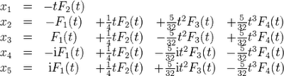
where

Just verifying one case:

>>> mp.dps = 25; mp.pretty = True
>>> t = mpf(3)
>>> for r in polyroots([1,0,0,0,-1,t]):
...     print r
... 
-1.341293531690699250693537
(0.9790618691253385511579325 - 0.6252190807348055061205923j)
(0.9790618691253385511579325 + 0.6252190807348055061205923j)
(-0.3084151032799889258111639 + 1.249926913731033699905407j)
(-0.3084151032799889258111639 - 1.249926913731033699905407j)
>>> -t*hyper(['1/5','2/5','3/5','4/5'], ['1/2','3/4','5/4'], 3125*t**4/256)
(-0.9790618691253385511579325 + 0.6252190807348055061205923j)

Now, we can choose t such that the hypergeometric argument becomes unity:

>>> t = root(mpf(256)/3125,4)
>>> for r in polyroots([1,0,0,0,-1,t]):
...     print r
... 
-1.103842268886161371052433
(0.6687403049764220240032331 + 3.167963942396665205386494e-14j)
(0.6687403049764220240032331 - 3.172324181973539074536523e-14j)
(-0.1168191705333413384770166 + 1.034453571405662514459057j)
(-0.1168191705333413384770166 - 1.034453571405662514459057j)
>>> -t*hyper(['1/5','2/5','3/5','4/5'], ['1/2','3/4','5/4'], 1)
-0.6687403049764220240032331

The last line would previously fail.

Interesting to note is that the value at the singular point z = 1 corresponds to a double root. This also makes polyroots return inaccurate values (note the imaginary parts), a known deficiency that should be fixed…

Better methods

In fact, there may be better methods than the Euler-Maclaurin formula. One such approach is to use the Abel-Plana formula, which I’ve also recently implemented as sumap(). The Abel-Plana formula gives the exact value for an infinite series (subject to some special growth conditions on the analytically extended summand) as a sum of two integrals.

The Abel-Plana formula is particularly useful when the summand decreases like a power of k; for example when the sum is a pure zeta function:

>>> sumap(lambda k: 1/k**2.5, [1,inf])
1.34148725725091717975677
>>> zeta(2.5)
1.34148725725091717975677
>>> sumap(lambda k: 1/(k+1j)**(2.5+2.5j), [1,inf])
(-3.385361068546473342286084 - 0.7432082105196321803869551j)
>>> zeta(2.5+2.5j, 1+1j)
(-3.385361068546473342286084 - 0.7432082105196321803869551j)

It actually works very well for the generalized hypergeometric series at the z = 1 singularity (which, as mentioned earlier, is a generalized polygamma function, polylogarithm, or zeta function of integer argument), and near the singularity as well. It should even be slightly faster than the Euler-Maclaurin formula since no derivatives are required. Yet another possibility is to integrate a Mellin-Barnes type contour for the hypergeometric function directly.

But at present, I don’t want to modify the existing hypergeometric code because it works and would only get more complicated. Rather, I want to improve nsum so it can handle all of this more easily without external hacks. The numerical integration code should also be improved first, because there are still certain parameter combinations where the hypergeometric function evaluation fails due to slow convergence in the numerical integration (this is due to an implementation issue and not an inherent limitation of the integration algorithm).

fredrikj.net | Blog index | RSS feed | Follow me on Mastodon | Become a sponsor