Post Sage Days 24 report

July 27, 2010

Now that I’ve overcome the immediate effects of SDWS (Sage Days Withdrawal Syndrome), I should write a brief report about Sage Days 24 which took place last week at the Research Institute for Symbolic Computation (RISC), located in a small town called Hagenberg just outside Linz in Austria. Many thanks for the organizers for inviting me!

Since I’m starting as a Ph.D. student at RISC in October, it was nice to get an early view of the site and meet some current students and staff. The location is quite beautiful, my only complaint being the extremely high temperature last week (they say the weather is more normal most of the year!).

SD24 was titled “Symbolic Computation in Differential Algebra and Special Functions”, which pretty accurately describes the topics covered. Some points of interest:

William Stein talked about his vision for Sage (short and long term), including goals for special functions support.

Frédéric Chyzak gave a talk about the Dynamic Dictionary of Mathematical Functions. I really like the approach of starting from a minimal definition of a special function (a differential equation with initial conditions) and generating series expansions, Chebyshev approximations (etc.) algorithmically.

Nico Temme talked about numerical evaluation of special functions, which was familiar grounds to me, but with much food for thought.

I met Manuel Kauers, my future supervisor, who gave a neat presentation of some recent research.

There were many other interesting talks and discussions as well, and I gave a talk about special function evaluation in mpmath (based on my SD23 talk). And of course, I met various other Sage developers and got some coding done as well.

I had hoped to get generalized hypergeometric functions into Sage during SD24. There is now a patch, but it still needs some more work.

I also implemented parabolic cylinder functions (PCFs) in mpmath, the last remaining chapter of hypergeometric functions listed in the DLMF (mpmath now covers chapters 1-20, 22, 24-25, partially 26-27, and 33). Code commit here.

Technically, parabolic cylinder functions are just scaled (linear combinations of) confluent hypergeometric functions or Whittaker functions, but they are a bit tricky to compute due to cancellation and branch cuts.

An example from Nico Temme’s talk was to evaluate D_ν(z) with ν = -300.14 and z = 300.15 (Maple 13 takes 5 seconds to give an answer that has the wrong sign and is off by 692 orders of magnitude). The new pcfd function in mpmath instantaneously (in about a millisecond) gives the correct result:

>>> pcfd(-300.14, 300.15)
6.83322814925713e-10526
>>> mp.dps = 30
>>> pcfd('-300.14', '300.15')
6.83322814923312844480669009487e-10526

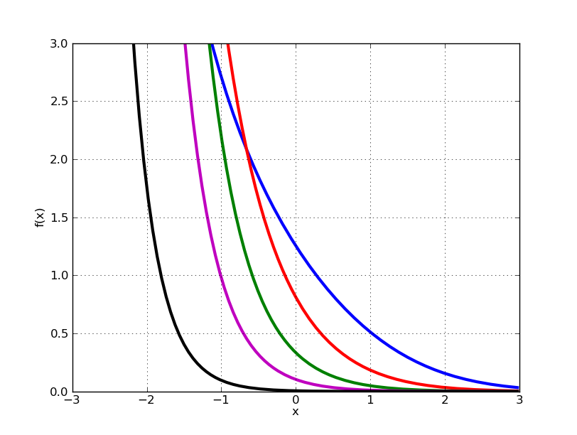
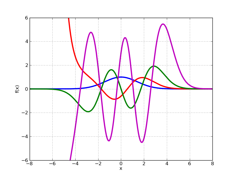
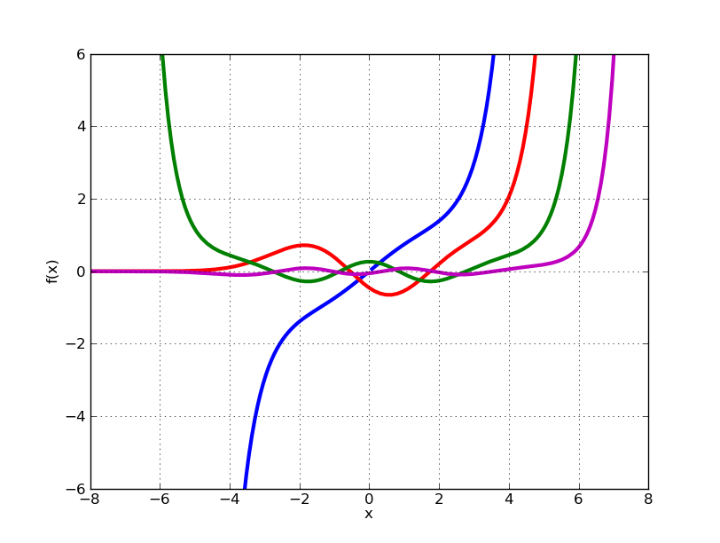
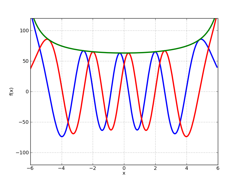
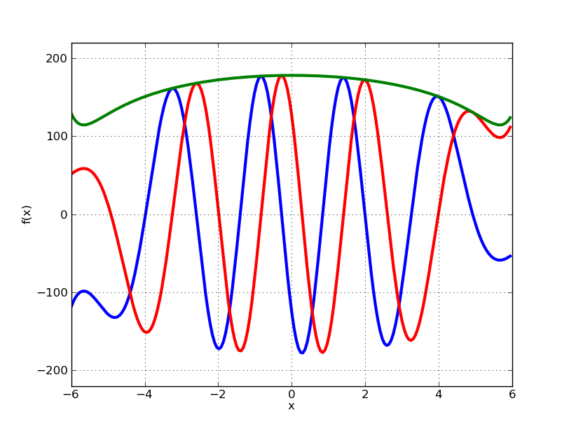
All the curve plots from DLMF 12.3can be reproduced as follows:

f1 = lambda x: pcfu(0.5,x)
f2 = lambda x: pcfu(2,x)
f3 = lambda x: pcfu(3.5,x)
f4 = lambda x: pcfu(5,x)
f5 = lambda x: pcfu(8,x)
plot([f1,f2,f3,f4,f5], [-3,3], [0,3])

f1 = lambda x: pcfv(0.5,x)
f2 = lambda x: pcfv(2,x)
f3 = lambda x: pcfv(3.5,x)
f4 = lambda x: pcfv(5,x)
f5 = lambda x: pcfv(8,x)
plot([f1,f2,f3,f4,f5], [-3,3], [-3,3])

f1 = lambda x: pcfu(-0.5,x)
f2 = lambda x: pcfu(-2,x)
f3 = lambda x: pcfu(-3.5,x)
f4 = lambda x: pcfu(-5,x)
plot([f1,f2,f3,f4], [-8,8], [-6,6])

f1 = lambda x: pcfv(-0.5,x)
f2 = lambda x: pcfv(-2,x)
f3 = lambda x: pcfv(-3.5,x)
f4 = lambda x: pcfv(-5,x)
plot([f1,f2,f3,f4], [-8,8], [-6,6])

f1 = lambda x: pcfu(-8,x)
f2 = lambda x: pcfv(-8,x)*gamma(0.5-(-8))
f3 = lambda x: hypot(f1(x), f2(x))
plot([f1,f2,f3], [-6,6], [-120,120])

f1 = lambda x: diff(pcfu,(-8,x),(0,1))
f2 = lambda x: diff(pcfv,(-8,x),(0,1))*gamma(0.5-(-8))
f3 = lambda x: hypot(f1(x), f2(x))
plot([f1,f2,f3], [-6,6], [-220,220])

A little more information can be found in the mpmath documentation section for PCFs.

Thanks again to the NSF grant enabling this work.

fredrikj.net | Blog index | RSS feed | Follow me on Mastodon | Become a sponsor