Embettered polynomial multiplication

April 17, 2014

With my thesis out of the way, I have time for coding again. Yay! First off my backlog has been to improve polynomial multiplication in FLINT and Arb.

Integer polynomials

FLINT generally multiplies integer polynomials using Kronecker substitution (KS): to compute $h = f g$, we choose a sufficiently large integer $k$, evaluate $f(2^k)$ and $g(2^k)$, compute the product $f(2^k) g(2^k)$, and then read off the coefficients of $h$ from the binary representation of the integer $h(2^k)$. KS reduces polynomial multiplication to a single (huge) integer multiplication, which GMP/MPIR does efficiently. Some bit twiddling is needed to pack/unpack the coefficients, but this only adds linear overhead.

KS is not used when either operand is very short (then classical $O(n^2)$ multiplication is faster), or when the polynomials have both high degree and large coefficients (then the Schönhage-Strassen algorithm is used). Previously, the cutoff between KS and classical multiplication was set to polynomials of degree 6.

Two weeks ago, I improved classical multiplication for the case when all input coefficients are "small" (commits 1, 2, 3, 4, 5, 6, 7). On a 64-bit system, the FLINT integer type (fmpz_t) stores values up to ± 2⁶²−1 = ± 4611686018427387903 directly, rather than as pointers to bignums. The default implementation of classical multiplication basically executes fmpz_addmul(z, x, y) or fmpz_addmul_ui(x, y, z) a total of $O(n^2)$ times. This means $O(n^2)$ times the overhead of (see the source code for fmpz_addmul_ui):

Calling a function
Checking that the input operands are small
Making case distinctions based on the signs
Doing the actual multiply-add operation
Determining whether the result is "small" or "big"
Storing the result

The idea to speed things up is very simple: do a single $O(n)$ pass to check if the input coefficients are all small and the output coefficients also are guaranteed to be small. In that case, we can do classical multiplication directly with the values, avoiding the overhead of steps 1-3 and 5-6.

void _fmpz_poly_mul_tiny1(fmpz * res, const fmpz * poly1,
                         slong len1, const fmpz * poly2, slong len2)
{
    slong i, j, c;

    _fmpz_vec_zero(res, len1 + len2 - 1);

    for (i = 0; i < len1; i++)
    {
        c = poly1[i];

        if (c != 0)
        {
            for (j = 0; j < len2; j++)
                res[i + j] += c * poly2[j];
        }
    }
}

This function works when both input and output coefficients have at most 62 bits. I also implemented a version for the case when the input coefficients are small and the output coefficients have at most 127 bits. In that case, we allocate a temporary array of two-word (128-bit) integers and execute the same algorithm with 64 x 64 → 128 bit multiplications and 128-bit additions.

The following plots compare performance when multiplying polynomials with 25-bit coefficients:

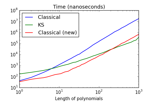
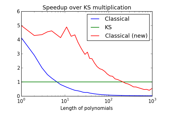
The speedup over the old multiplication code is biggest around length 10, where we gain a factor five. This is nice and expected, but I was surprised to find that the cutoff for KS multiplication suddenly jumps very high – from lengths less than 10 to over 200 with coefficients of this particular size! For fmpz_poly_mullow (truncating multiplication), the cutoff can be as high as 400.

The speedup also varies slightly depending on the size of the input coefficients, as illustrated in the following plot:

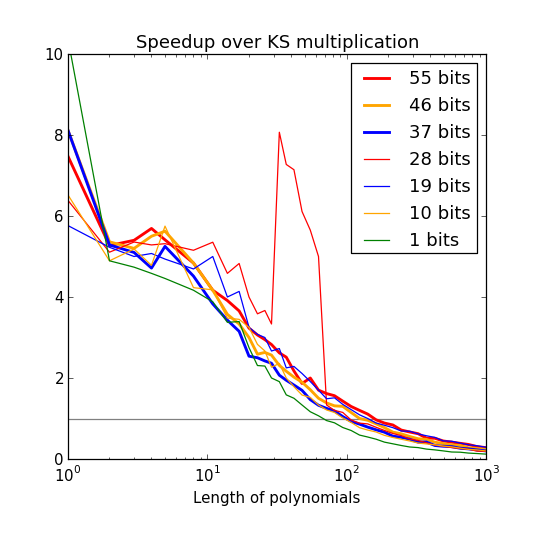
Polynomial multiplication speedup, different bit sizes

In general, KS has an advantage for smaller coefficients since it can pack several coefficients into each word, but even with 1-bit coefficients, the cutoff is around 50. How can it be so high? This basically comes down to linear overhead. Packing or unpacking a single word-size coefficient takes something like 10 nanoseconds. The code for this could be tightened, but probably not by much: you have to read the data, do the bit shifting, and complement sign-extended values, while handling word boundaries and other edge cases. Meanwhile, a single-word multiply-add can be done in something like 1 nanosecond. Thus, a 40 x 40 classical multiplication with the new code takes about 1600 nanoseconds, which is the amount of time that it takes just to pack and unpack the coefficients for the corresponding KS multiplication, i.e. (40 + 40 + 80) x 10 = 1600 nanoseconds.

There is a curious jump with 28-bit coefficients, which occurs precisely between length 32 and 63. Here the coefficients actually just barely fit in 62 bits when using signed integers, but KS multiplication uses the bound 63 bits since it needs one extra bit to encode the sign using twos complement. This makes the bit unpacking code promote each output coefficient to a bignum and then demote it again. This could clearly be improved.

I have carefully inserted cutoffs so that fmpz_poly_mul, fmpz_poly_mullow, fmpz_poly_sqrmul and fmpz_poly_sqrlow automatically select the fastest algorithm for nearly any combination of lengths and bit sizes, at least on Sandy Bridge CPUs (the cutoffs should obviously be tuned for different architectures).

It remains to be seen whether this speeds up any real-world computations. A nice test problem involving multivariate polynomial arithmetic is the Fateman benchmark, which is to compute the product $f \times (f + 1)$ where $f$ is a power of a sum of monomials. FLINT currently doesn't do multivariate polynomial arithmetic directly, but we can represent multivariate polynomials recursively using univariate polynomials at the bottom (using bland). This is the result for the multiplication:

Polynomial	Old time (s)	New time (s)
$f = (x+y+z+1)^{20}$	0.050	0.028
$f = (x+y+z+1)^{30}$	0.62	0.29
$f = (x+y+z+t+1)^{10}$	0.023	0.014
$f = (x+y+z+t+1)^{20}$	2.97	1.46
$f = (x+y+z+t+1)^{30}$	57.65	27.9

We get a 2x speedup across the board. Note that this is just doing lots of univariate multiplications recursively; it is not doing anything clever for multivariate polynomials (such as multivariate Kronecker substitution).

Real polynomials

I discussed polynomial multiplication with real and complex coefficients in Arb last year: here and here. There are two core problems: dealing with coefficients of varying magnitude, and implementing error propagation. The classical $O(n^2)$ multiplication algorithm, using ball arithmetic, automatically works equally well regardless of the coefficient magnitudes (giving nearly optimal accuracy and nearly optimal propagated error bounds). But this algorithm is also slow. It is generally better to rescale the polynomial so that it has integer coefficients (possibly breaking it into smaller blocks first) and multiplying using fmpz_poly functions.

Error propagation works as follows: if the input polynomials are $(A, \varepsilon_{A})$ and $(B, \varepsilon_{B})$ (where $\varepsilon_{A}$ and $\varepsilon_{B}$ are polynomials representing the errors of the midpoint polynomials $A$, $B$), we need to compute an upper bound for $|A| |\varepsilon_{B}| + |B| |\varepsilon_{A}| + |\varepsilon_{A}| |\varepsilon_{B}|$ where the absolute value signs apply coefficient-wise. We can do this very quickly by just taking norm bounds, but this becomes horrible when the coefficients vary in magnitude (consider the power series for $\exp(x)$: $10^{-100}$ would be a good error bound for the first coefficient, but a horrible bound for the coefficient of $x^{1000}$, $1/1000! \approx 10^{-2568}$).

To compute accurate propagated error bounds for all coefficients, we basically need three polynomial multiplications instead of one (note that we can collect terms to make it three instead of four). A factor three is a rather high price to pay! But fortunately, the cost can usually be made much smaller in practice, since the error bounds don't need very high precision.

Previously, I implemented error propagation essentially using classical multiplication with 1-bit arithmetic, representing each coefficient by a power of two. This algorithm is $O(n^2)$ but with a very small implied constant (just a couple of cycles per operation). Up to length $n = 10000$ or so, the cost was usually negligible, although it did start to get slow for much longer polynomials. But the bigger problem was that the slight overestimation tended to cause blowup. With 100-bit precision and length-1000 polynomials, say, a single multiplication might overestimate the error by a factor 1000 (roughly the same order of magnitude as the degree), i.e. giving 90-bit accuracy. So for a single multiplication, just increasing the precision by 10 bits is sufficient to get a good error bound. But when doing a sequence of multiplications where each result depends on the previous one, the overestimation adds up exponentially. Of course, this problem is inherent to interval or ball arithmetic, but the 1-bit precision made the problem much worse than necessary in practice.

So, this week I reimplemented polynomial multiplication in Arb to fix these flaws (commit 1, 2). To make a long story short, the new code contains two improvements. For very long blocks of coefficients, it uses fmpz_poly_t multiplication (the same algorithm as used to multiply the midpoints of polynomials) instead of classical multiplication. For short blocks of coefficients (up to length 1000), it does $O(n^2)$ multiplication using doubles instead of powers-of-two. This is about as fast as the old code (also just a couple of cycles per operation), but gives several digits of accuracy.

Of course, this has to be done very carefully. Doubles only have a range between roughly $2^{-1024}$ and $2^{1024}$, and the coefficients of bignum polynomials generally do not fit in this range. But there is a workaround: the same code that is used to split polynomials into blocks of similarly-sized coefficients to make fmpz_poly multiplication efficient can be used to split polynomials into blocks in which all coefficients fit a double when multiplied by a common power of two. Another problem is that the arithmetic operations done on doubles can end up rounding down instead of up. Fortunately, all numbers are nonnegative, so there can be no catastrophic cancellation: it is sufficient to do floating-point arithmetic as usual and in the end multiply by a factor close to unity (say, 1.000001) to get an upper bound.

When it comes to "real-world" problems that I've used Arb for, such as computing Keiper-Li coefficients and Swinnerton-Dyer polynomials, the new multiplication code generally makes no difference in terms of speed, and just gives slightly better accuracy. It's possible to construct input where it's slightly slower than the old code. But it's also easy to find examples where the improvement is dramatic. Here is one: let $f$, $g$ be the length-$n$ Taylor polynomials of $\sin(x)$ and $\cos(x)$ respectively. Computing the power series quotient $f / g$ gives us the Taylor polynomial for $\tan(x)$. The following table shows the timing for this division as well as the coefficient of $x^{n-1}$ in the output:

n	Time (old)	Value (old)	Time (new)	Value (new)
10	0.000028 s	0.0218694885361552 +/- 3.473e-17	0.000022 s	0.0218694885361552 +/- 2.6561e-20
30	0.00011 s	2.61477115129075e-06 +/- 5.2042e-17	0.00097 s	2.61477115129075e-06 +/- 2.3173e-23
100	0.00066 s	4.88699947810437e-20 +/- 1.6544e-22	0.00066 s	4.88699947810437e-20 +/- 5.3731e-36
300	0.0042 s	2.91787636775164e-59 +/- 1.5661e-51	0.0042 s	2.91787636775164e-59 +/- 3.1382e-74
1000	0.041 s	1.51758479114333e-196 +/- 3.1587e-173	0.040 s	1.51758479114333e-196 +/- 1.2975e-210
3000	0.38 s	8.73773572457598e-589 +/- 4.465e-502	0.37 s	8.73773572457598e-589 +/- 9.5225e-602
10000	4.44 s	1.26549284530317e-1961 +/- 2.6516e-1597	4.29 s	1.26549284530317e-1961 +/- 1.3072e-1973
30000	44.4 s	5.06662884259426e-5884 +/- 5.2199e-5099	42.6 s	5.06662884259426e-5884 +/- 3.6094e-5895
100000	543 s	2.05743905925107e-19612 +/- 1.6689e-16560	523 s	2.05743905925107e-19612 +/- 1.8036e-19622

Note that both before and after, the midpoints are computed accurately, but the error bounds are wildly different. With the old multiplication, we supposedly only know two correct digits when $n = 100$, and no digits at all when $n = 300$. When $n = 10000$, the error bound is too large by more than a factor $10^{384}$. With the new algorithm, we only lose one digit of accuracy per row of the table!

In the previous example, the magnitude variation causes the complexity to degenerate to $O(n^2)$ (since many short blocks have to be used). The new code gives a huge improvement when multiplying polynomials which have all coefficients of the same magnitude. For example, if we multiply the Taylor series for $\log(1+x)$ and $\operatorname{atan}(x)$ at a precision of 256 bits, the following happens:

n	Time (old)	Value (old)	Time (new)	Value (new)
10	0.000027 s	-0.048015873015873 +/- 6.5311e-77	0.000030 s	-0.048015873015873 +/- 3.5984e-78
30	0.000061 s	-0.0151107262962829 +/- 9.7292e-77	0.000066 s	-0.0151107262962829 +/- 2.7088e-78
100	0.00027 s	-0.0115365985205729 +/- 8.1099e-77	0.00027 s	-0.0115365985205729 +/- 1.1699e-78
300	0.0011 s	-0.00379706290713168 +/- 6.0757e-77	0.0011 s	-0.00379706290713168 +/- 4.3993e-79
1000	0.0054 s	-0.00113410736253996 +/- 1.0122e-76	0.0043 s	-0.00113410736253996 +/- 2.0084e-79
3000	0.028 s	-0.000377560938223733 +/- 7.5908e-77	0.015 s	-0.000377560938223733 +/- 6.6569e-80
10000	0.22 s	-0.000113218498717764 +/- 6.3254e-77	0.061 s	-0.000113218498717764 +/- 2.139e-80
30000	1.7 s	-3.77347607812753e-05 +/- 9.488e-77	0.24 s	-3.77347607812753e-05 +/- 9.6506e-81
100000	17 s	-1.13199307375816e-05 +/- 7.9067e-77	0.76 s	-1.13199307375816e-05 +/- 2.9353e-81

The new code is softly linear instead of quadratic; at $n = 100000$, the speedup is a factor 20.

P.S. embetter is a perfectly cromulent word.

fredrikj.net | Blog index | RSS feed | Follow me on Mastodon | Become a sponsor