fredrikj.net / blog /
The 2F1 bites the dust
October 19, 2015
The Gauss hypergeometric function ${}_2F_1(a,b,c,z)$ is finally in Arb. This versatile function has many applications in physics, statistics, and other fields. Its special cases include:
- Legendre and Jacobi polynomials, and their generalizations to complex orders (e.g. the Legendre functions $P_{\lambda}^{\mu}(z)$, $Q_{\lambda}^{\mu}(z)$)
- The incomplete beta function $B(z;\,a,b) = \int_0^z t^{a-1}\,(1-t)^{b-1}\,dt = z^a{}_2F_1(a,1-b;a+1;z) / a$
- Inverse trigonometric functions and complete elliptic integrals (of course, these functions are best computed by less general methods, as Arb indeed does)
Previously, the Gauss hypergeometric function could mostly be computed using the tools available in Arb for generalized hypergeometric series, but you had to piece those tools together for different cases (and some corner cases require further work, as discussed below). My project this weekend was to put everything together. The code commits are: 1, 2, 3, 4, 5, 6.
Algorithm
The Gauss hypergeometric function is the analytic continuation of the hypergeometric series $${}_2F_1(a,b,c,z) = \sum_{k=0}^{\infty} \frac{(a)_k (b)_k}{(c)_k} \frac{z^k}{k!}$$ which converges for $|z| < 1$ for generic values of the parameters $a, b, c$ (for special integer values of the parameters, the series might terminate after a finite number of terms, and it might not exist at all when $c = 0, -1, -2, \ldots$). Arb also implements the regularized hypergeometric function $\mathop{\mathbf{F}}(a,b,c,z) = {}_2F_1(a,b,c,z) / \Gamma(c)$, which exists even when $c$ is a nonpositive integer.
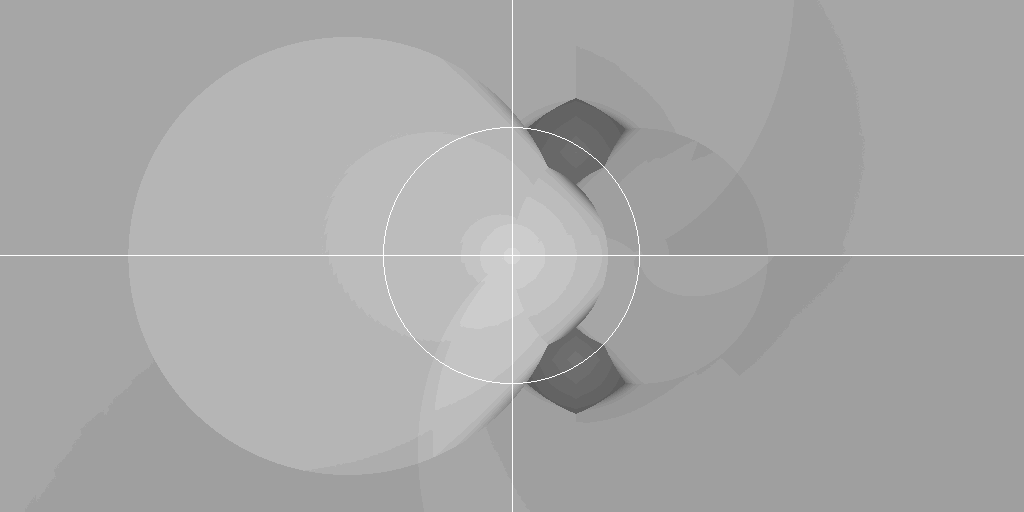
The hypergeometric series is effective for computation when $|z| < 0.75$, say. For larger $|z|$, one can try to apply a linear fractional transformation to the argument (section 15.8 in the DLMF). A ${}_2F_1$ of argument $z \not\in \{0,1,\infty\}$ can always be transformed into a ${}_2F_1$ or a sum of two ${}_2F_1$'s of argument $$\frac{z}{z-1}, \quad \frac{1}{z}, \quad \frac{1}{1-z}, \quad 1-z, \quad 1-\frac{1}{z}.$$ For example, the $z \to 1/z$ formula reads $$ \frac{\sin(\pi(b-a))}{\pi} \mathbf{F}(a,b,c,z) = \frac{(-z)^{-a}}{\Gamma(b)\Gamma(c-a)} \mathbf{F}\!\left(a,a-c+1,a-b+1,\frac{1}{z}\right) - \frac{(-z)^{-b}}{\Gamma(a)\Gamma(c-b)} \mathbf{F}\!\left(b,b-c+1,b-a+1,\frac{1}{z}\right).$$ Generally speaking, the goal is to choose the linear fractional transformation that results in the smallest absolute value, but there are also other factors affecting efficiency; for example, when sticking to $z$ or $z/(z-1)$, there is just one series to evaluate instead of two, and no extra gamma function values are required. The following picture shows how Arb currently chooses between $z$ (green), $z/(z-1)$ (aquamarine), $1/z$ (red), $1/(1-z)$ (blue), $1-z$ (yellow), $1-1/z$ (orange). The unit circle and the real and imaginary axes are drawn in white.

The black regions are the difficult corner cases. All transformations leave the points $\exp(\pm \pi i / 3) = \tfrac{1}{2} (1 \pm \sqrt{3} i)$ fixed (or simply swap them). Near these points, the hypergeometric series converges too slowly to be used for numerical evaluation, regardless of which argument transformations have been applied. Macsyma, Mathematica and others (including mpmath) solve this problem by switching to an algorithm by Bill Gosper. However, I currently don't have rigorous error bounds for this method. It's also possible to use standard convergence acceleration methods. Again, I don't have error bounds for such methods, so I can't use them at the moment.
My solution in Arb is to analytically continue the function using the hypergeometric differential equation $$z(1-z) F''(z) + \left[c-(a+b+1)z \right] F'(z) - ab F(z) = 0,$$ starting from initial values obtained at a point where the hypergeometric series converges rapidly. For high-precision integration of this ODE, local Taylor expansions are effective. I use the Cauchy-Kovalevskaya majorant method to obtain error bounds. The Cauchy-Kovalevskaya method is actually a powerful tool for showing the existence of solutions of partial differential equations, but it allows determining explicit local bounds as a nice side effect (for a refined and more general version of this method to compute bounds, see the paper Effective bounds for P-recursive sequences by Marc Mezzarobba and Bruno Salvy). The error bounds can become quite bad when the parameters $a,b,c$ are large, but overall this works decently.
The analytic continuation code in Arb currently performs two integration steps ($0.375 \pm 0.625i \to 0.5 \pm 0.8125i \to z$), which is a very simplistic way to do it. The algorithm could be optimized for high precision and rational parameters by taking a sequence of decreasing steps (this leads to the asymptotically fast "bit-burst" algorithm when done correctly).
Limit cases
When applying transformation formulas, a problem arises: one ends up dividing by a factor $\sin(\pi(b-a))$ or $\sin(\pi(c-a-b))$, which becomes zero when $b-a$ or $c-a-b$ is an integer. Thus, one has to compute the limit $$\lim_{\varepsilon \to 0} {}_2F_1(a + \varepsilon,b,c,z).$$
There are different ways to do this. In mpmath, I settled for computing the limit numerically, effectively by setting $\varepsilon$ to a finite but nonzero value (e.g. roughly $2^{-53}$ at 53-bit precision). I don't want to do this in Arb, for three reasons: it would defeat potential future high-precision optimizations, it would would give far too wide output intervals in some cases, and most importantly, I don't have rigorous error bounds for this method.
The more robust way is to compute the limit formally. In reference works, one can find ugly-looking formulas for the limiting cases of the ${}_2F_1$ involving infinite series of digamma functions. However, we don't need these series expansions explicitly (in particular, there's no need to do a separate error analysis for each such infinite series). Instead, we can implement the normal transformations for ${}_2F_1$ using arithmetic in $\mathbb{C}[[\varepsilon]] / \langle \varepsilon^2 \rangle$, that is, with dual numbers. Evaluating the convergent hypergeometric series with power series as parameters is already implemented in Arb. Now computing the limit $\lim_{\varepsilon \to 0} {}_2F_1(a + \varepsilon,b,c,z)$ is just an application of L'Hôpital's rule. No ugly special limit formulas required!
The full picture
A simple test is to plot ${}_2F_1(0.2+0.3i, 0.4+0.5i, 0.5+0.6i, z)$ on $z \in [-4,4] + [-2,2]i$ at a resolution of 1024 times 512 pixels. For plotting, 64-bit precision is more than enough. The following plot takes 200 seconds to produce with Arb, which is six times faster than mpmath (1260 seconds) at the same precision (with the simpler parameters $1/4, 1/2, 1$ instead, Arb takes 60 seconds, which is 14 times faster than mpmath).

It's interesting to check how much accuracy we lose, considering that the input parameters are inexact intervals (for example, $0.2$ is parsed as $[3689348814741910323 \cdot 2^{-64} \pm 2^{-66}]$) and that the error bounds grow when doing a sequence of interval operations. The following plot uses brightness to indicate the number of accurate bits divided by 64; that is, white would represent full 64-bit accuracy in the output and black would represent complete loss of accuracy. The loss of accuracy generally turns out to be around 5-12 bits except near $\exp(\pm \pi i / 3)$ where up to 23 bits are lost. This is probably improvable, but it's not too shabby.
High-precision benchmarks
I did a few tests to compare mpmath and Arb on my laptop which has a 1.90 GHz Intel i5-4300U CPU. I've also included timings for Mathematica 9.0 on a 3.07 GHz Intel Xeon X5675 CPU.
Easy case
${}_2F_1(1/2,1/4,1,z)$ at $z = \sqrt{5} + \sqrt{7} i$. The parameters are simple numbers, the $1/z$ transformation gives rapid convergence, and no limit has to be computed. As a side note, with these parameters, the function is equivalent to an elliptic integral, which can be used as an independent check of correctness. I use 20 guard bits with Arb to get a result with full accuracy.
| Digits | Mathematica | mpmath | Arb |
| 10 | 0.00066 s | 0.00090 s | 0.00011 s |
| 100 | 0.0039 s | 0.0017 s | 0.00075 s |
| 1000 | 0.23 s | 1.5 s | 0.019 s |
| 10000 | 42.6 s | 98 s | 1.2 s |
Corner case
${}_2F_1(1/2,1/4,1,z)$ at $z = \exp(\pi i / 3)$. It's clear that the algorithm in Arb could be optimized.
| Digits | Mathematica | mpmath | Arb |
| 10 | 0.00050 s | 0.0048 s | 0.00060 s |
| 100 | 0.0056 s | 0.031 s | 0.0046 s |
| 1000 | 0.17 s | 0.46 s | 0.16 s |
| 10000 | 30 s | 51 s | 29 s |
Limit case
${}_2F_1(10+i,5+i,1,z)$ at $z = \sqrt{5} + \sqrt{7} i$. Here, a limit has to be computed when applying the $1/z$ transformation since $a-b$ is an integer, which slows things down.
| Digits | Mathematica | mpmath | Arb |
| 10 | 0.0025 s | 0.0060 s | 0.00066 s |
| 100 | 0.016 s | 0.10 s | 0.0042 s |
| 1000 | 0.46 s | 27 s | 0.26 s |
| 10000 | 108 s | - | 56 s |
A precision challenge
We compute $\log(-\operatorname{Re}[{}_2F_1(500i, -500i, -500 + 10^{-500}i, 3/4)])$ accurately. Here's a friendly reminder that Mathematica's N[] cannot be trusted (to be fair, the same warning applies to any software).
Mathematica 9.0 for Linux x86 (64-bit)
Copyright 1988-2013 Wolfram Research, Inc.

In[1]:= $MaxExtraPrecision = 10^6;

In[2]:= Timing[N[Log[-Re[Hypergeometric2F1[500I, -500I, -500 + 10^(-500) I, 3/4]]], 10]]
Out[2]= {0.372000, 2697.176919}

In[3]:= Timing[N[Log[-Re[Hypergeometric2F1[500I, -500I, -500 + 10^(-500) I, 3/4]]], 20]]
Out[3]= {0.004000, 2697.1769189940809154}

In[4]:= Timing[N[Log[-Re[Hypergeometric2F1[500I, -500I, -500 + 10^(-500) I, 3/4]]], 50]]
Out[4]= {0.004000, 2697.1769189940809154478570904365185898022661405959}

In[5]:= Timing[N[Log[-Re[Hypergeometric2F1[500I, -500I, -500 + 10^(-500) I, 3/4]]], 100]]
Out[5]= {0.004000, 2697.17691899408091544785709043651858980226614059592813667681109698158446822885085\
>     6831149308154069600}

In[6]:= Timing[N[Log[-Re[Hypergeometric2F1[500I, -500I, -500 + 10^(-500) I, 3/4]]], 200]]
Out[6]= {0.356000, 2697.17691899408091544785709043651858980226614059592813667681109698158446822885085\
>     68311493081540696004092616280278261394279337920572811364380682810646743000974280124760540266927\
>     404954014134808667401452}

In[7]:= Timing[N[Log[-Re[Hypergeometric2F1[500I, -500I, -500 + 10^(-500) I, 3/4]]], 500]]
Out[7]= {76.484000, 2003.5749041098714598611978336159150450496846561380225356317831875334900609058895\
>     41655266120646349997384148511115997598121423048884454074086968893329058260435047844278223319968\
>     81952851038218673251970825702246408166178242147908137636167517153977217295526620201331126724266\
>     71076314732871666757724374886020543566995468740274547609599114847423758014504261912509791664290\
>     52480061657539062451835078476837784539517551640451980850278901845935590889147733825974806746031\
>     0381754198923206283681742160842269698809}
Mathematica gives a completely wrong value when we ask for 10, 20, 50, 100 or even 200 digits, and then suddenly gives the correct value when we ask for 500 digits!
With Arb, adaptive numerical evaluation can be done with a code snippet such as the following:
for (prec = 64; ; prec *= 2)
{
    arb_set_str(acb_realref(a), "0.0", prec);
    arb_set_str(acb_imagref(a), "500.0", prec);
    arb_set_str(acb_realref(b), "0.0", prec);
    arb_set_str(acb_imagref(b), "-500.0", prec);
    arb_set_str(acb_realref(c), "-500.0", prec);
    arb_set_str(acb_imagref(c), "1e-500", prec);
    arb_set_str(acb_realref(z), "0.75", prec);
    arb_set_str(acb_imagref(z), "0.0", prec);

    acb_hypgeom_2f1(w, a, b, c, z, 0, prec);
    arb_zero(acb_imagref(w));
    acb_neg(w, w);
    acb_log(w, w, prec);

    if (acb_rel_accuracy_bits(w) > 3.33 * digits)
    {
        arb_printn(acb_realref(w), digits, 0); printf(" + ");
        arb_printn(acb_imagref(w), digits, 0); printf("i\n");
        break;
    }
}
It computes correct results:
digits = 10
[2003.574904 +/- 1.10e-7] + 0i
cpu/wall(s): 0.68 0.679

digits = 20
[2003.5749041098714599 +/- 3.89e-17] + 0i
cpu/wall(s): 0.686 0.686

digits = 50
[2003.5749041098714598611978336159150450496846561380 +/- 2.26e-47] + 0i
cpu/wall(s): 0.713 0.713

digits = 100
[2003.5749041098714598611978336159150450496846561380225356317831875334900609058895
41655266120646349997 +/- 3.85e-97] + 0
cpu/wall(s): 0.712 0.712

digits = 200
[2003.5749041098714598611978336159150450496846561380225356317831875334900609058895
4165526612064634999738414851111599759812142304888445407408696889332905826043504784
42782233199688195285103821867325197083 +/- 4.30e-197] + 0i
cpu/wall(s): 2.36 2.359

digits = 500
[2003.5749041098714598611978336159150450496846561380225356317831875334900609058895
4165526612064634999738414851111599759812142304888445407408696889332905826043504784
4278223319968819528510382186732519708257022464081661782421479081376361675171539772
1729552662020133112672426671076314732871666757724374886020543566995468740274547609
5991148474237580145042619125097916642905248006165753906245183507847683778453951755
1640451980850278901845935590889147733825974806746031038175419892320628368174216084
2269698809 +/- 4.35e-497] + 0i
cpu/wall(s): 2.45 2.448
With mpmath, the following can be used. Like Mathematica, this is just a heuristic, and it could fail, but it happens to give correct results in this case:
>>> F = autoprec(lambda: log(-re(hyp2f1(500j,-500j,"-500+1e-500j",0.75,maxprec=10**6))))
>>> mp.dps = 10; print timing(F), F()
6.65178203583 2003.574904
>>> mp.dps = 20; print timing(F), F()
6.50600981712 2003.5749041098714599
>>> mp.dps = 50; print timing(F), F()
6.64240193367 2003.574904109871459861197833615915045049684656138
>>> mp.dps = 100; print timing(F), F()
5.93264389038 2003.574904109871459861197833615915045049684656138022535631783187533
490060905889541655266120646349997
>>> mp.dps = 200; print timing(F), F()
5.54282307625 2003.574904109871459861197833615915045049684656138022535631783187533
4900609058895416552661206463499973841485111159975981214230488844540740869688933290
582604350478442782233199688195285103821867325197083
>>> mp.dps = 500; print timing(F), F()
16.4163320065 2003.574904109871459861197833615915045049684656138022535631783187533
4900609058895416552661206463499973841485111159975981214230488844540740869688933290
5826043504784427822331996881952851038218673251970825702246408166178242147908137636
1675171539772172955266202013311267242667107631473287166675772437488602054356699546
8740274547609599114847423758014504261912509791664290524800616575390624518350784768
3778453951755164045198085027890184593559088914773382597480674603103817541989232062
83681742160842269698808
To do
The ${}_2F_1$ implementation can still be improved in many ways. It's not yet optimized for high precision in many cases. For certain combinations of large parameters, choosing transformations that result in smaller parameters would be worthwhile. Performance could certainly be improved near $z = \exp(\pm \pi i \sqrt{3})$, especially when $a, b, c$ are large. Finally, the code is not currently designed for rational parameters $a, b, c$. It happens to work well for denominators 1, 2, 4, 8 and so on which are exact in a floating-point representation, but parameters like $1/3$ or $1/10$ are not supported optimally at the moment.
fredrikj.net |
Blog index |
 RSS feed |
Follow me on Mastodon |
Become a sponsor
RSS feed |
Follow me on Mastodon |
Become a sponsor