fredrikj.net / blog /
Airy in the library
November 20, 2015
Airy functions, named after the British astronomer and mathematician George Biddell Airy, are solutions of the following second-order ODE:
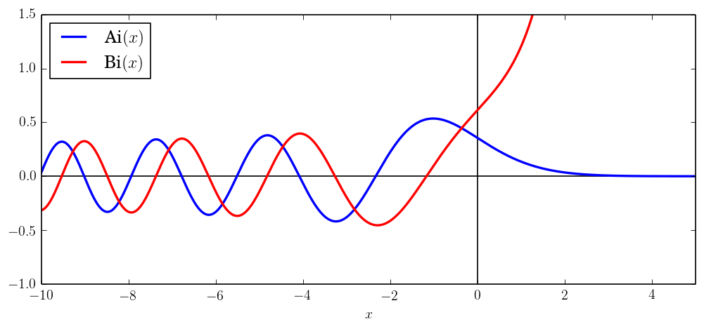
$$f''(x) = x f(x).$$ The Airy equation is the prototypical ODE with a turning point. Consider the following ODEs and their respective solutions: $$f''(x) = +f(x), \quad f(x) = C_1 \exp(x) + C_2 \exp(-x)$$ $$f''(x) = -f(x), \quad f(x) = C_1 \sin(x) + C_2 \cos(x)$$When $x > 0$, the Airy equation resembles the first equation: the solutions either increase or decrease exponentially. When $x < 0$, the Airy equation resembles the second equation: the solutions oscillate like sines and cosines.
The general solution of the Airy equation is $C_1 \operatorname{Ai}(x) + C_2 \operatorname{Bi}(x)$, where Ai and Bi are two special solutions which have been defined so that Ai is decreasing and Bi is increasing to the right of the turning point at $x = 0$.
Airy functions are useful in asymptotic analysis of differential equations, and they show up in a huge number of applications in physics. One of the textbook examples in quantum mechanics is the one-dimensional stationary Schrödinger equation for a particle in a linear potential, $$\left[ \frac{-\hbar^2}{2\mu}\nabla^2 + (V(x) - E) \right] \Psi(x) = 0, \quad V(x) = C x,$$ which is equivalent to the Airy equation after a change of variables.
Implementation in Arb
Airy functions can be expressed in terms of Bessel functions or confluent hypergeometric functions of orders $n \pm 1/3$. In particular, $$\operatorname{Ai}(z) = \frac{1}{3^{2/3} \Gamma(2/3)} {}_0F_1\left(\frac{2}{3}, \frac{z^3}{9}\right) - \frac{z}{3^{1/3} \Gamma(1/3)} {}_0F_1\left(\frac{4}{3}, \frac{z^3}{9}\right)$$ $$\operatorname{Bi}(z) = \frac{1}{3^{1/6} \Gamma(2/3)} {}_0F_1\left(\frac{2}{3}, \frac{z^3}{9}\right) + \frac{3^{1/6} z}{\Gamma(1/3)} {}_0F_1\left(\frac{4}{3}, \frac{z^3}{9}\right).$$
The Airy functions could have been implemented rather easily by wrapping the pre-existing Bessel functions or confluent hypergeometric functions in Arb, but I decided to do a more elaborate implementation from scratch instead (main commit).Why? First of all, the pre-existing Bessel and hypergeometric code is less than optimal for order $n \pm 1/3$ (fractions with power-of-two denominators are more efficient due to being exact). Even if I were to fix this deficiency, going via other special functions would still involve a lot of redundant computation. I also wanted to make the Airy functions numerically stable everywhere, meaning that the error bounds for the output should be close to the best possible, given a nonzero error bound for the input. This is currently not the case for Bessel functions in Arb. Obviously, I want to make the Bessel functions more numerically stable too, but that is a much harder project for the future!
The implementation of Airy functions in Arb (acb_hypgeom_airy and its helper functions) comprises some 2000 lines of code including unit tests and documentation, and has the following features:
- The input $z$ is a complex interval. The code supports arbitrary precision and gives rigorous error bounds (obviously).
- Any combination of the four functions $\operatorname{Ai}(z), \operatorname{Ai}'(z), \operatorname{Bi}(z), \operatorname{Bi}'(z)$ can be computed simultaneously (like sine and cosine, they are often used together, and this is faster than performing 2-4 independent function evaluations).
- For small and exact $z$, the convergent ${}_0F_1$ series are used. The working precision is automatically increased to compensate for catastrophic cancellation.
- For small and inexact $z$, the functions are evaluated at the midpoint of $z$, and accurate propagated error bounds are computed using derivative bounds obtained from asymptotic expansions.
- For large $z$, asymptotic expansions are used directly. This is automatically numerically stable.
- Hardware double-precision arithmetic is used to quickly determine whether asymptotic expansions can be used, and to compute tight estimates of the number of terms to use and the working precision needed to overcome cancellation. This is a heuristic step, and error bounds are subsequently computed rigorously using interval arithmetic and directed rounding.
- Both the convergent and asymptotic series are evaluated using an efficient rectangular splitting strategy to reduce the number of costly multiplications.
Note that while only the zeroth and first order derivatives are computed, both Ai and Bi satisfy $$f^{(2)}(z) = z f(z)$$ $$f^{(n+3)}(z) = z f^{(n+1)}(z) + (n+1) f^{(n)}(z),$$ so computing the higher derivatives is a simple exercise for the user. I might add convenience functions later for evaluating Airy functions of power series.
Asymptotic expansions
I will elaborate on how asymptotic functions are used, because this bit was somewhat painful to work out in detail. The math is simple; the difficulty was to get the error bounds right everywhere, including corner cases where the input is an interval straddling more than one region, and implementing everything in verbose C code with redundant steps optimized out.
First, recall that for a given tolerance $2^{-p}$, asymptotic expansions can be used only when $|z|$ is sufficiently large. For given $z$ and $p$, how do we find out whether asymptotic expansions give sufficient accuracy, and how many terms to use? If we denote the terms in the asymptotic expansion by $t(n)$, the easiest way is to simply estimate $\log_2 |t(0)|, \log_2 |t(1)|, \ldots$. We can proceed to use the asymptotic series when we find an $n$ such that $\log_2 |t(n)| < -p$. If we run into an $n$ such that $\log_2 |t(n)| > \log_2 |t(n-1)|$, the asymptotic series will not give sufficient accuracy, so we abort and use a convergent series instead. (This strategy is too simplistic for asymptotic series in general, but it works here.) This initial "parameter selection stage" can use cheap hardware arithmetic, as rigorous error bounds will be computed later.
I used the bounds derived by Frank Olver and presented in his chapter on Airy functions in the DLMF. The starting point is the asymptotic expansion for $\operatorname{Ai}(z)$ in the direction $z \to +\infty$, which actually is valid as $|z| \to \infty$ along any complex ray other than the negative half of the real line. With $\zeta = (2/3) z^{3/2}$, we have $$\operatorname{Ai}(z) = \frac{e^{-\zeta}}{2 \sqrt{\pi} z^{1/4}} \left[S_n(\zeta) + R_n(z)\right]$$ where $$S_n(\zeta) = \sum_{k=0}^{n-1} (-1)^k \frac{u(k)}{\zeta^k}, \quad u(k) = \frac{(1/6)_k (5/6)_k}{2^k k!}.$$
Olver gives an explicit bound for the error term $R_n(z)$. This bound deteriorates with increasing $\arg(z)$, as I have indicated in the figure below on the left. We get very good bounds for $|\arg(z)| < \pi / 3$ (green), just slightly worse bounds for $\pi / 3 < |\arg(z)| < 2 \pi / 3$ (yellow), worse but still usable bounds for $2 \pi / 3 < |\arg(z)| \ll \pi$ (orange), and near $|\arg(z)| = \pi$, the bounds blow up (red). We want to use this asymptotic expansion in the green sector if possible, and in the yellow sector otherwise. The orange sector can be used if there are no other options, and in that case we should try to stay close to the transition line between the yellow and orange sectors.
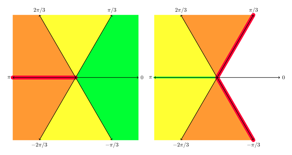
Left: quality of asymptotic expansion for $\operatorname{Ai}(z)$. Right: quality of asymptotic expansions for $\operatorname{Ai}(z), \operatorname{Bi}(z)$ using connection formulas.
Now the idea, as suggested by Olver, is to derive asymptotic expansions for other cases using connection formulas. For $z$ in the left half-plane, we can use
$$\operatorname{Ai}(z) = e^{+\pi i/3} \operatorname{Ai}(z_1) + e^{-\pi i/3} \operatorname{Ai}(z_2)$$ $$\operatorname{Bi}(z) = e^{-\pi i/6} \operatorname{Ai}(z_1) + e^{+\pi i/6} \operatorname{Ai}(z_2)$$ where $z_1 = -z e^{+\pi i/3}$ and $z_2 = -z e^{-\pi i/3}$. These connection formulas rotate the argument by one-third of a turn. Taking the asymptotic expansions of both the Airy functions on the right hand side, and combining terms, we get an expansion whose overall quality is the worse of the two. This is indicated in the picture above to the right. Explicitly, $$\operatorname{Ai}(z) = A_1 [S_n(i \zeta) + R_n(z_1)] + A_2 [S_n(-i \zeta) + R_n(z_2)]$$ $$\operatorname{Bi}(z) = A_3 [S_n(i \zeta) + R_n(z_1)] + A_4 [S_n(-i \zeta) + R_n(z_2)]$$ where $\zeta = (2/3) (-z)^{3/2}$ and $$ A_1 = \frac{\exp(-i (\zeta - \pi/4))}{2 \sqrt{\pi} (-z)^{1/4}}, \quad A_2 = \frac{\exp(+i (\zeta - \pi/4))}{2 \sqrt{\pi} (-z)^{1/4}}, \quad A_3 = -i A_1, \quad A_4 = +i A_2.$$ Note that, although the connection formulas are valid for all $z$, the combined asymptotic expansion is only valid for $|\arg(-z)| < 2 \pi / 3$ (due to the branch cuts of the prefactor).As a special case, looking at the negative half real axis in the picture above to the right, $\operatorname{Ai}(x)$ and $\operatorname{Bi}(x)$ with $x < 0$ become linear combinations of $\operatorname{Ai}(-x e^{\pm \pi i/3})$, lying on the transition lines between the yellow and green regions in the picture on the left.
The remaining case to handle is for Bi in the right half plane. Here we use the connection formulas $$\operatorname{Bi}(z) = -i (2 \omega^{+1} \operatorname{Ai}(z \omega^{-2}) - \operatorname{Ai}(z))$$ $$\operatorname{Bi}(z) = +i (2 \omega^{-1} \operatorname{Ai}(z \omega^{+2}) - \operatorname{Ai}(z))$$ where $\omega = \exp(\pi i/3)$. Combining roots of unity gives $$\operatorname{Bi}(z) = \frac{1}{2 \sqrt{\pi} z^{1/4}} [2X + iY]$$ $$\operatorname{Bi}(z) = \frac{1}{2 \sqrt{\pi} z^{1/4}} [2X - iY]$$ $$\zeta = (2/3) z^{3/2}, \quad X = \exp(+\zeta) [S_n(-\zeta) + R_n(z \omega^{\mp 2})], \quad Y = \exp(-\zeta) [S_n(\zeta) + R_n(z)]$$ where the upper formula is valid for $-\pi/3 < \arg(z) < \pi$ and the lower formula is valid for $-\pi < \arg(z) < \pi/3$, as illustrated in the following picture. We therefore use the upper formula when the midpoint of the complex interval $z$ lies in the upper half plane and the lower formula when the midpoint lies in the lower half plane (exactly on the real line, the choice is arbitrary).
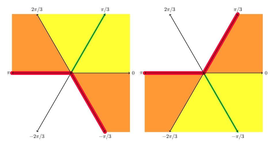
Quality of asymptotic expansions for Bi in the right half plane.
Note that, in all cases, we we only need to evaluate $S_n(\zeta)$ and $S_n(-\zeta)$ with the same $\zeta$ to compute both Ai and Bi.
The formulas can be rearranged using trigonometric prefactors instead of exponentials. This makes everything real for negative real numbers, whereas the current formulas use alternating real and imaginary numbers there. Error bounds can also be simplified for purely real input: when the series are real and alternating, the error term is always bounded by the first omitted term. I might implement these improvements in the future.
Benchmarking
For real arguments, we can compare performance with the mpfr_ai function in MPFR and airyai in mpmath. At 64-bit precision, Arb computes $\operatorname{Ai}(x)$ in 10-20 microseconds. This is about twice as fast as MPFR when $x$ is small. When $x$ grows larger, MPFR becomes progressively worse since it does not use asymptotic expansions. The plot below clearly shows the two peaks in running time where Arb switches to asymptotic expansions.
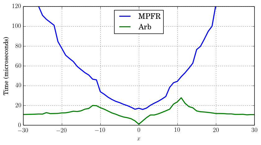
Time to compute $\operatorname{Ai}(x)$ at 64-bit precision.
Although mpmath uses asymptotic expansions and thus holds up decently for large arguments, it is much slower overall. The following plot shows, zoomed out, how many times faster Arb is compared to both MPFR and mpmath:
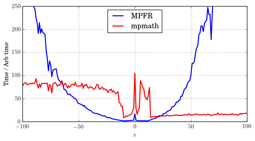
Relative to compute $\operatorname{Ai}(x)$ at 64-bit precision.
At 3333-bit precision (approximately 1000 digits), Arb computes $\operatorname{Ai}(x)$ in 2-5 milliseconds. This is again consistently faster than both MPFR and mpmath. The algorithm selection in mpmath is evidently very poorly tuned at high precision, slowing down so much that it goes off the scale in the following picture for $4 < x < 145$. Interestingly, though, mpmath is almost as fast as Arb for very large positive $x$ at this precision.
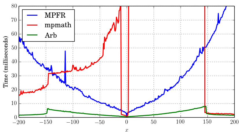
Time to compute $\operatorname{Ai}(x)$ at 3333-bit precision.
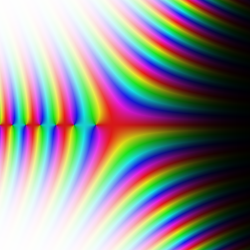
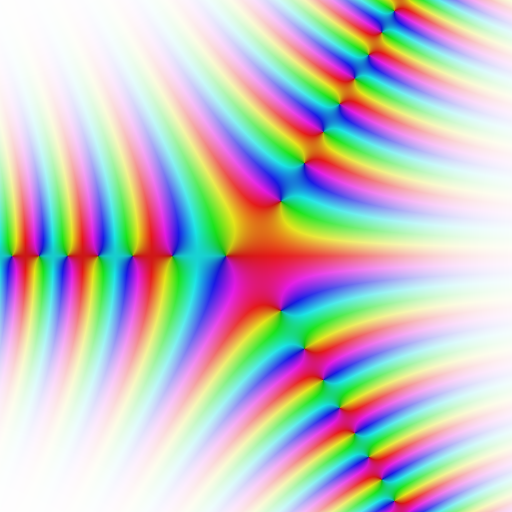
Complex arguments
Complex arguments are uniformly 2-3 times slower than real arguments at the same precision. The following 512 × 512 pixel domain colored plots of $\operatorname{Ai}(z)$ (left) and $\operatorname{Bi}(z)$ (right) for $z \in [-10,10] + [-10,10]i$ take 4.5 seconds to render, using a precision of 32 bits.
Airy function zeros
The Airy functions have an infinite sequence of real zeros $\operatorname{Ai}(a_n) = 0$, $\operatorname{Ai}'(a'_n) = 0$, $\operatorname{Bi}(b_n) = 0$, $\operatorname{Bi}'(b'_n) = 0$. The first few are (to 10 digits):
| $n$ | $a_n$ | $a'_n$ | $b_n$ | $b'_n$ |
| 1 | −2.338107410 | −1.018792972 | −1.173713223 | −2.294439683 |
| 2 | −4.087949444 | −3.248197582 | −3.271093303 | −4.073155089 |
| 3 | −5.520559828 | −4.820099211 | −4.830737842 | −5.512395730 |
| 4 | −6.786708090 | −6.163307356 | −6.169852128 | −6.781294446 |
| 5 | −7.944133587 | −7.372177255 | −7.376762079 | −7.940178689 |
I have added the Airy functions to the real_roots example program in Arb. The root isolation code in real_roots is completely generic; it relies purely on being able to evaluate the object function and its derivatives in interval arithmetic. No information about the asymptotic distribution of the Airy function zeros is being exploited (the real_roots program also demonstrates computing zeros of the Riemann zeta function, among other things).
As an example, it takes 0.42 seconds to isolate the 6710 zeros of Ai on the interval $[-1000,0]$:
> build/examples/real_roots 4 -1000 0
interval: [-1000, 0]
maxdepth = 30, maxeval = 100000, maxfound = 100000, low_prec = 30
---------------------------------------------------------------
Found roots: 6710
Subintervals possibly containing undetected roots: 0
Function evaluations: 67630
cpu/wall(s): 0.422 0.422
virt/peak/res/peak(MB): 26.53 26.62 2.84 2.84
It takes 22 seconds to refine the same roots to 1000 digits each, using the generic interval-based Newton implementation in the real_roots program:
> build/examples/real_roots 4 -1000 0 -refine 1000
interval: [-1000, 0]
maxdepth = 30, maxeval = 100000, maxfound = 100000, low_prec = 30
refined root (0/6710):
[-999.91936797636384994814500357673698631708289035752812949732355246454007214238
25086529843391546979436196231893145318672911388387266290425955036381424104232098
21959382653054011888556159446303334635494058949724054670914786934157812832725621
48570812584692491527774337420208731102210790047229476074274853394924213976700895
97580436794894052812227037752689570656407403587710732355191345956498354320530151
18660106942295153080293923850567984960731493151090629784038685434639197165625890
85130653019088783348634739791224364373594066461909106531257454732410908834151192
38802875549281404703161420778764091123067337625555878759094759769005544736642007
89167465389486941290248512307222405921246839935100788138798415264483876537498881
25098099674593190356753322787295530107789755304296202511420183179820218581298845
86769916429662702945835883728795767839498403812110277990163911791399981306024793
52085495485976709757632171720364376730208389565085957359416676037020290396839781
305110544033095396544333692750290268350505130 +/- 4.50e-1000]

     (... long output omitted ...)

refined root (6709/6710):
[-2.3381074104597670384891972524467354406385401456723878524838544372136680027002
83647782164041731329320284760093853265952775225466858359866744868898716819727540
97315267499111274806599964562835349155036724215460225304014264499417846393445344
44576009473858055993284003541978854868734370327947683736231269144363684562163216
95224896886771887967253644542964146651161756655217909281106701616013124010872087
51068015363540930435540173336518243684153688846153833781673263744772352166269178
98162900770617327677839962800890838040518659518893258577111583822210212170758191
40042838771579610361895347743266687702532274665250544694660076354855478498996553
85449531527883777571079976665872920752336809007511567307314992020073711012994084
30413874201048355826398350502612457374298884716015896813993360718225735302714533
73298042317302785618884411551002742408721103590746604387755833964377689014281692
08537738426486491923178234284354349366643196163933956066902105416207641584372042
297422983703788795834149300831159961531707775 +/- 3.12e-1002]

---------------------------------------------------------------
Found roots: 6710
Subintervals possibly containing undetected roots: 0
Function evaluations: 221960
cpu/wall(s): 22.593 22.891
virt/peak/res/peak(MB): 26.53 26.62 2.84 2.84
For comparison, mpmath takes 800 seconds to compute the same roots at low precision (by repeatedly calling mpmath.airyaizero), and an estimated 8000 seconds at 1000-digit precision. I tested Mathematica's AiryAiZero as well (on a different machine), and it takes 2.8 and 264 seconds respectively.
Returning to the Schrödinger equation, the $a_n$ are precisely the possible energy values of a quantum mechanical particle in a linear potential well, expressed in appropriate dimensionless units. (The $a'_n$ can also be energy values, depending on boundary conditions.) On a tangent to this, the late Richard Crandall wrote an interesting paper on so-called quantum zeta functions (On the quantum zeta function [PDF], J. Phys. A: Math. Gen. 29 (1996) 6795-6816). These are formal sums $$Z(s) = \sum_{k=1}^{\infty} \frac{1}{E_k^s}$$ where $E_k$ are the energy states of a fixed quantum system. The Airy zeta functions are $$Z(s) = \sum_{k=1}^{\infty} \frac{1}{a_k^s}, \quad z(s) = \sum_{k=1}^{\infty} \frac{1}{|a_k|^s}.$$ Remarkably, like the Riemann zeta function in the famous Basel problem, these functions have simple closed forms at the positive even integers $s = 2, 4, 6, \ldots$. For example, $$Z(2) = \frac{3^{5/3} \Gamma^4(2/3)}{4 \pi^2}.$$ Perhaps even more remarkably, Crandall conjectured special values for the analytic continuations of $z(s)$ and $Z(s)$, in particular $$z(1) \stackrel{?}{=} -\frac{\Gamma(2/3)}{3^{2/3} \Gamma(4/3)}.$$ This is, as far as I know, still an open conjecture!
fredrikj.net |
Blog index |
 RSS feed |
Follow me on Mastodon |
Become a sponsor
RSS feed |
Follow me on Mastodon |
Become a sponsor