fredrikj.net / blog /
Arb 2.11 is available
July 10, 2017
Arb version 2.11 is now available. The changelog this time is quite short, but it includes a few nice additions. There are actually many other improvements in the pipeline, but they will not be ready until later this year, and there was no good reason to delay incrementing the version number. Here is the changelog for 2.11.0, with more detail about the major new features below.
- Special functions
- Added the Lambert W function (arb_lambertw, acb_lambertw, arb_poly_lambertw_series, acb_poly_lambertw_series). All complex branches and evaluation of derivatives are supported.
- Added the acb_expm1 method, complementing arb_expm1.
- Added arb_sinc_pi, acb_sinc_pi.
- Optimized handling of more special cases in the Hurwitz zeta function.
- Polynomials
- Added the arb_fmpz_poly module to provide Arb methods for FLINT integer polynomials.
- Added methods for evaluating an fmpz_poly at arb_t and acb_t arguments.
- Added arb_fmpz_poly_complex_roots for computing the real and complex roots of an integer polynomial, turning the functionality previously available in the poly_roots.c example program into a proper library function.
- Added a method (arb_fmpz_poly_gauss_period_minpoly) for constructing minimal polynomials of Gaussian periods.
- Added arb_poly_product_roots_complex for constructing a real polynomial from complex conjugate roots.
- Miscellaneous
- Fixed test code in the dirichlet module for 32-bit systems (contributed by Pascal Molin).
- Use flint_abort() instead of abort() (contributed by Tommy Hofmann).
- Fixed the static library install path (contributed by François Bissey).
- Made arb_nonnegative_part() a publicly documented method.
- Arb now requires FLINT version 2.5 or later.
Note: a patched version 2.11.1 was released immediately after 2.11.0 to fix a FLINT version compatibility issue.
The Lambert W function
The Lambert W function $W_k(z)$ is the multivalued inverse function of $f(w) = w e^w$. It often turns up in asymptotic analysis (for instance in saddle point approximations and inverse estimates of the gamma function), so it is a very useful standard function for a mathematical library. Arb now supports computing the two real branches $W_{0}$ and $W_{-1}$ via arb_lambertw, and arbitrary complex branches $W_k$ via acb_lambertw. In addition arb_poly_lambertw_series and acb_poly_lambertw_series allow computing the Lambert W function of power series.
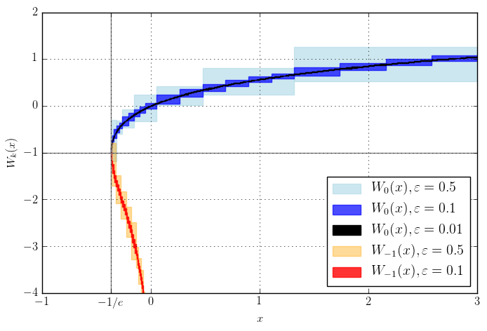
Plot of the real branches $W_0(x)$ and $W_{-1}(x)$ computed with Arb. The boxes show the size of the output intervals given wide input intervals. In this plot, the input intervals have been subdivided until the output radius is smaller than $\varepsilon$.
The general approach to compute the Lambert W function is to solve $w e^w - z = 0$ using a Newton-like root-finding algorithm. So far very simple, but in practice things get very complicated when we insist on rigorous error bounds, being able to compute all the branches (and provably ending up on precisely the branch the user asked for!), supporting arbitrary precision, handling very large or small arguments, and allowing the input $z$ to be inexact. This blog post will not go into a lot of detail, because I've already written up a technical paper, available on arXiv: Computing the Lambert W function in arbitrary-precision complex interval arithmetic.
In Arb, I implemented a two-stage algorithm: the function is first approximated using double arithmetic, which gives nearly 53 correct bits, but not provably so. This nonrigorous approximation is subsequently refined (if necessary) and certified using arbitrary-precision arithmetic. At low precision, this strategy is extremely fast since we only need to do a single refinement and certification step with arbitrary-precision arithmetic. To complicate matters, arbitrary-precision code is still needed for the initial approximation very close to branch points or when when the input would overflow or underflow the double exponent range. This extra code adds a lot of implementation complexity. Nonetheless, the speedup due to the separate double code path for "normal" input is well worth the trouble.
At low precision, computing the Lambert W function of a real argument takes about $10^{-6}$ seconds, while a complex argument takes about $10^{-5}$ seconds. The following table shows the relative time to compute $w = W_0(z)$ compared to that of computing $e^w$, at a precision of 10, 100, 1000 and 10000 decimal digits. We see that the Lambert W function is not much slower than elementary functions.
| $z$ | 10 | 100 | 1000 | 10000 |
| $10$ | 3.36 | 7.12 | 1.60 | 1.50 |
| $10^{10}$ | 3.64 | 6.92 | 1.65 | 1.53 |
| $10^{10^{20}}$ | 3.46 | 8.39 | 1.91 | 1.67 |
| $10i$ | 13.20 | 8.68 | 4.71 | 3.27 |
| $-10^{10^{20}}$ | 3.69 | 29.75 | 7.53 | 4.59 |
| $-1/e+10^{-100}$ | 4.57 | 2.33 | 2.23 | 1.97 |
| $-1/e-10^{-100}$ | 4.43 | 2.36 | 7.08 | 2.89 |
For power series, a simple test case is $h(x) = W_0(e^{1+x})$. Using 256-bit precision, arb_poly_lambertw_series takes 2.8 seconds to compute this series expansion to length 10001, giving $$[x^{10000}] h(x) \in [-6.02283194399026390 \cdot 10^{-5717} \pm 5.56 \cdot 10^{-5735}]$$ or if we multiply by $10000!$, the derivative $$h^{(10000)}(0) \in [-1.714254372711877171 \cdot 10^{29943} \pm 7.78 \cdot 10^{29924}].$$
Anecdote 1: to get good error bounds in the algorithm for the Lambert W function, I needed to prove some inequalities for $|W_k(z)|$ and $|W_k'(z)|$. Some steps were done using explicit interval computations with Arb (bootstrapped from independent bounds to avoid circularity of course!). For example, here is a plot of the Lambert W function on a closed loop around the branch point at $z = -1/e$, which is used to get an error bound for the Puiseux expansion:
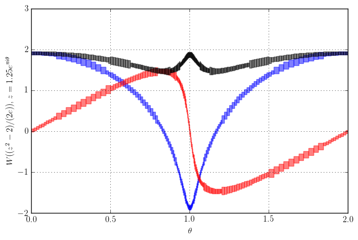
Plot of the real (blue) and imaginary (red) part and the absolute value (black) of $2 + W((z^2-2)/(2e)), z = 1.25 e^{\pi i \theta}$ with continuous analytic continuation. The function argument $(z^2-2)/(2e)$ traces two loops around the branch point at $-1/e$. From left to right, the branch cycles through $W_0, W_1, W_{-1}, W_0$. Input intervals have been subdivided adaptively to show that the absolute value is bounded by 2.
Anecdote 2: while testing the Lambert W implementation, I noticed that the special value $$W_2\left(-\frac{9\pi}{2}\right) = \frac{9 \pi}{2} i = 14.1371669\ldots i$$ approximates the imaginary component of the smallest nontrivial zero of the Riemann zeta function to within a relative error of 2 parts in 10000. Is this just a numerical coincidence, or are the lizard people taking over?
Methods for FLINT polynomials
By popular demand, Arb has gained an arb_fmpz_poly module for using FLINT integer polynomials (fmpz_poly_t) together with Arb real and complex numbers.
For example, this module provides the methods arb_fmpz_poly_evaluate_arb and arb_fmpz_poly_evaluate_acb to evaluate a FLINT integer polynomial directly at a real or complex argument. Previously, this required converting the polynomial an arb_poly_t, which is wasteful unless the same polynomial is to be evaluated several times.
Most importantly, this module provides the method arb_fmpz_poly_complex_roots which computes all the real and complex roots of an integer polynomial. The code is exactly that of the old poly_roots.c example program, but the functionality is now exposed as a convenient library function instead of forcing the user to copy and paste a huge chunk of code.
The root-finding code has some nice features: it always separates the purely real roots from the complex roots (which are separated into conjugate pairs), and it automatically reduces the degree of polynomials of the form $f(x^n)$. The algorithm can still be improved a lot, especially for real root isolation, but it should be good enough for most applications.
Gaussian period minimal polynomials
Jean-Pierre Flori explained the following algorithm to me and suggested that I implement it in Arb during the 8th Atelier PARI/GP last month. A surprising application of complex arithmetic is to construct finite extension fields $GF(p^n)$ for given prime $p$ and degree $n > 1$. This amounts to finding an irreducible polynomial $f \in (\mathbb{Z}/p\mathbb{Z})[x]$ of degree $n$. The obvious way to find such a polynomial is to generate random degree-$n$ polynomials and perform an irreducibility test on each candidate. However, there exist special polynomials which are guaranteed to be irreducible over $(\mathbb{Z}/p\mathbb{Z})[x]$, without the need to perform an explicit irreducibility test!
One such family of special polynomials are the minimal polynomials of Gaussian periods, which are certain sums over roots of unity (chosen appropriately for a given $p$ and $n$). To construct an irreducible polynomial using Gaussian periods, we first find a prime $q$ such that $q-1 = nd$ and such that $n$ is coprime with $(q-1)/f$ where $f$ is the multiplicative order of $p$ mod $q$. Then the polynomial $$f = (x-r_0)(x-r_2) \cdot (x-r_{n-1}) \in \mathbb{Z}[x], \quad r_k = \sum_{j=0}^{d-1} \zeta^{g^{k+nj}}$$ is irreducible mod $p$, where $g$ is a primitive root mod $q$ and $\zeta = \exp(2\pi i / q)$.
Here is a concrete numerical example: given $p = 17, n = 8$, a cheap brute force search finds the parameters $q = 41, d = 5, g = 6$. Then $$r_0 = \zeta^{1} + \zeta^{10} + \zeta^{18} + \zeta^{16} + \zeta^{78} \in [0.1455208873131 \pm 6.36 \cdot 10^{-14}] + [1.5866563192184 \pm 4.29 \cdot 10^{-14}] i$$ $$r_1 = \zeta^{6} + \zeta^{60} + \zeta^{26} + \zeta^{14} + \zeta^{58} \in [-2.4359328700651 \pm 5.53 \cdot 10^{-14}] + [1.6269772641436 \pm 7.69 \cdot 10^{-14}] i $$ $$r_2 = \zeta^{36} + \zeta^{32} + \zeta^{74} + \zeta^{2} + \zeta^{20} \in [1.2052601720451 \pm 6.75 \cdot 10^{-14}] + [-2.238011017337 \pm 1.19 \cdot 10^{-13}] i$$ $$r_3 = \zeta^{52} + \zeta^{28} + \zeta^{34} + \zeta^{12} + \zeta^{38} \in [0.5851518107069 \pm 3.47 \cdot 10^{-14}] + [-0.2770801200416 \pm 5.29 \cdot 10^{-14}] i$$ and so on (in fact, $r_4, r_5, r_6, r_7$ are just the complex conjugates of the first four roots). Expanding the factorization of $f$ with Arb arithmetic gives $$f \in x^8 + [1.00000000000 \pm 2.59 \cdot 10^{-13}] x^7 + [3.00000000000 \pm 2.65 \cdot 10^{-12}] x^6$$ $$+ [11.0000000000 \pm 9.74 \cdot 10^{-12}] x^5 + [44.0000000000 \pm 2.93 \cdot 10^{-11}] x^4$$ $$+ [-53.0000000000 \pm 4.64 \cdot 10^{-11}] x^3 + [153.0000000000 \pm 6.55 \cdot 10^{-11}] x^2$$ $$+ [-160.0000000000 \pm 4.82 \cdot 10^{-11}] x + [59.0000000000 \pm 1.65 \cdot 10^{-11}]$$ so we conclude that $$f = x^8 + x^7 + 3 x^6 + 11 x^5 + 44 x^4 - 53 x^3 + 153 x^2 - 160 x + 59.$$ Reducing the coefficients mod 17, we obtain $$GF(17^8) \cong GF(17)[x] / (x^8 + x^7 + 3x^6 + 11x^5 + 10x^4 + 15x^3 + 10x + 8).$$
This is not-so-coincidentally the same polynomial that Pari/GP produces when asked to construct a finite field:
? ffinit(17, 8)
%1 = Mod(1, 17)*x^8 + Mod(1, 17)*x^7 + Mod(3, 17)*x^6 + Mod(11, 17)*x^5 + Mod(10, 17)*x^4 + Mod(15, 17)*x^3 + Mod(10, 17)*x + Mod(8, 17)
The Pari/GP implementation (which is due to Bill Allombert) indeed uses Gaussian periods, but it uses $\ell$-adic arithmetic instead of complex arithmetic, to avoid issues with rounding errors (though it actually uses complex arithmetic to estimate the magnitude of the coefficients and hence the needed $\ell$-adic precision). With Arb, we use complex arithmetic directly and still get a certified result.
Here are some timings (in seconds) for Pari/GP's ffinit versus Arb's arb_fmpz_poly_gauss_period_minpoly.
| $p$ | $n$ | Pari/GP | Arb |
| 17 | 27 = 128 | 0.008 | 0.00143 |
| 17 | 28 = 256 | 0.031 | 0.00595 |
| 17 | 29 = 512 | 0.049 | 0.0196 |
| 17 | 210 = 1024 | 0.152 | 0.0795 |
| 17 | 211 = 2048 | 0.492 | 0.266 |
| 17 | 212 = 4096 | 2.891 | 1.992 |
| 17 | 213 = 8192 | 11.163 | 13.368 |
| 17 | 214 = 16384 | 47.0 | 25.6 |
| 17 | 215 = 32768 | 176 | 95 |
| 2607−1 | 35 = 243 | 0.003 | 0.00292 |
| 2607−1 | 36 = 729 | 0.031 | 0.0183 |
| 2607−1 | 37 = 2187 | 0.348 | 0.28 |
| 2607−1 | 38 = 6561 | 4.485 | 3.557 |
| 2607−1 | 39 = 19683 | 35.8 | 22.2 |
| 2607−1 | 310 = 59049 | 944 | 566 |
Both approaches are comparable, with Arb generally being just slightly faster. A notable feature of the algorithm is that increasing $p$ barely affects the running time (in sharp contrast to irreducibility testing). The reason for only using prime power $n$ in the benchmark, by the way, is that it is faster to handle general $n$ via compositums of prime power degrees instead of using Gaussian periods directly (Pari/GP uses this trick in ffinit).
Arb uses a baby-step giant-step scheme to compute the roots of unity (this functionality was implemented recently by Pascal Molin) as well as a fast tree for the polynomial expansion, which are key tricks to making the implementation really fast. I have not studied the Pari/GP source code carefully, but I believe that it uses essentially the same tricks (only with $\ell$-adic arithmetic instead of complex arithmetic).
fredrikj.net |
Blog index |
 RSS feed |
Follow me on Mastodon |
Become a sponsor
RSS feed |
Follow me on Mastodon |
Become a sponsor