fredrikj.net / blog /
Announcing Python-FLINT 0.2
November 1, 2018
I'm pleased to announce version 0.2 of Python-FLINT, the Python wrapper for FLINT and Arb.
Python-FLINT gives Python users access to highly efficient arbitrary-precision integers, rationals, real and complex numbers (using Arb's rigorous ball arithmetic), and highly efficient matrices, polynomials and power series over all these base types. It goes beyond basic arithmetic by wrapping a wide range of FLINT and Arb features, from polynomial factorization and root-finding to special functions and rigorous numerical integration. Quick example:
>>> from flint import *
>>> ctx.dps = 30
>>> acb.integral(lambda x, _: (-x**2).exp(), -100, 100) ** 2
[3.141592653589793238462643383 +/- 3.11e-28]
More examples are given below in this post.
General information
In contrast to Sage which wraps FLINT and Arb but also comes with a huge list of other dependencies and generally has its own ways of doing things, Python-FLINT is just a small standalone Python extension module, designed to be used in ordinary Python sessions along with other libraries. It has far fewer features than Sage, but it can be a more convenient solution for users who don't need the full power of a computer algebra system. The interface in Python-FLINT is also a bit simpler (for example, there is no need to construct parent rings) and Python-FLINT sometimes provides more complete access to the underlying libraries.
Here is a quick link to a Google Colab notebook demonstrating how easy Python-FLINT is to install and use. There is just one small problem at the moment: Arb has to be compiled and installed from source, which takes a few minutes (Arb 2.15 is required, and the apt-get version is too old). Once FLINT and Arb are installed, Python-FLINT itself only takes a minute to install with pip install python-flint. I hope to see a CoCalc demo notebook soon as well.
I started Python-FLINT in 2012, resurrected it in 2015, and have now (appropriate for the season) resurrected it again. I hope it will remain alive (not just undead) this time! Python-FLINT was originally just a hack for myself to test FLINT functions from the comfort of a REPL, and I never had the time to work on making it a proper library for other people to use. When people asked me, I usually recommended some other solution instead. However, an increasing number of people have reminded me that Python-FLINT could be useful to them if it was in better shape, so I finally put in the work. I apologize for not having done this much earlier!
The 0.2 release is the first version that is really usable and maintainable as a library. Most imporantly, both Python 2 and Python 3 now work, several minor issues have been fixed, more automatic conversions are supported (for example between Arb and mpmath types), more test code and documentation has been added, and Travis CI testing has finally been set up (giving me peace of mind). In terms of features, I have focused on wrapping useful Arb functionality. Version 0.2 is now largely up to date with Arb 2.15, although there are still some unwrapped Arb functions. I have not had time to wrap more FLINT features apart from a handful of matrix methods; finite fields are still notably absent.
With that said, some highlights follow:
Reliable linear algebra
A nice application of Python-FLINT is to solve ill-conditioned linear systems, where ordinary numerical software might struggle. Consider $Ax = b$ where $A$ is the Hilbert matrix $(A_{i,j} = 1/(i+j+1))$ of size $n$ and $b$ is a vector of ones. What is entry $\lfloor n/2 \rfloor$ in the solution vector $x$? Here are the answers according to SciPy and mpmath (at default precision):
>>> from mpmath import mp
>>> from scipy import matrix, ones
>>> from scipy.linalg import hilbert, det, solve
>>> for n in range(1,20):
...     a = solve(hilbert(n), ones(n))[n//2]
...     b = mp.lu_solve(mp.hilbert(n), mp.ones(n,1))[n//2,0]
...     print("%i   %.10g %.10g" % (n, a, b))
...
1   1 1
2   6 6
3   -24 -24
4   -180 -180
5   630 630
6   5040.000001 5040
7   -16800.00006 -16800.00005
8   -138600.0038 -138599.9984
9   450448.7578 450448.5854
10   3783740.267 3783408.229
11   -12120268.65 -12084254.18
12   -107176657.1 -101153955.3
13   159846382.8 1537346756
14   -375101334.6 -405911178.6
15   -61205732.51 -3927346.364
16   2621798308 229589156.9
17   2091986643 -141126648.9
18   -543467386.4 -708788796.2
19   -1401092752 -339671743.5
The solutions to the exact problem are integers, but already at $n = 9$, both SciPy and mpmath give answers that are not close to integers (the nearest integer to both answers, 450449, is also off by one from the correct solution). At $n = 14$ the answers from SciPy and mpmath are clearly diverging, indicating that something is wrong, but in fact even for $n = 13$ the two common leading digits in both answers are wrong!
We could get better answers out of mpmath by increasing the precision, but this still leaves us with the problem of figuring out how much precision will be sufficient. Now let us try the same calculations with Arb matrices, also at standard (53-bit) precision:
>>> from flint import *
>>> for n in range(1,20):
...     print("%i    %s" % (n, arb_mat.hilbert(n,n).solve(arb_mat(n,1,[1]*n))[n//2,0]))
...
1    1.00000000000000
2    [6.00000000000000 +/- 5.78e-15]
3    [-24.00000000000 +/- 1.65e-12]
4    [-180.000000000 +/- 4.87e-10]
5    [630.00000 +/- 1.03e-6]
6    [5040.00000 +/- 2.81e-6]
7    [-16800.000 +/- 3.03e-4]
8    [-138600.0 +/- 0.0852]
9    [4.505e+5 +/- 57.5]
10    [3.78e+6 +/- 6.10e+3]
11    [-1.2e+7 +/- 3.37e+5]
Traceback (most recent call last):
  File "", line 2, in
  File "src/arb_mat.pyx", line 402, in flint.arb_mat.solve (src/pyflint.c:102965)
ZeroDivisionError: singular matrix in solve()
Arb gives error bounds and raises an exception when it cannot prove that the matrix is invertible, so we know precisely when higher precision is needed. The user can easily write a loop that increases the precision until the result is good enough. In fact, the builtin Python-FLINT function good() implements precisely such a loop:
>>> f = lambda: arb_mat.hilbert(n,n).solve(arb_mat(n,1,[1]*n), nonstop=True)[n//2,0]
>>> for n in range(1,20):
...     good(f)
...
1.00000000000000
[6.00000000000000 +/- 2e-19]
[-24.0000000000000 +/- 1e-18]
[-180.000000000000 +/- 1e-17]
[630.000000000000 +/- 2e-16]
[5040.00000000000 +/- 1e-16]
[-16800.0000000000 +/- 1e-15]
[-138600.000000000 +/- 1e-14]
[450450.000000000 +/- 1e-14]
[3783780.00000000 +/- 3e-13]
[-12108096.0000000 +/- 3e-12]
[-102918816.000000 +/- 3e-11]
[325909584.000000 +/- 3e-11]
[2793510720.00000 +/- 3e-10]
[-8779605120.00000 +/- 3e-9]
[-75724094160.0000 +/- 3e-8]
[236637794250.000 +/- 3e-8]
[2050860883500.00 +/- 3e-7]
[-6380456082000.00 +/- 3e-7]
(Above, nonstop=True was inserted to return a matrix instead of raising ZeroDivisionError which interrupts good().)
Here is a bigger example, requiring several hundred bits of precision:
>>> n = 100
>>> good(f, verbose=True)
prec = 53, maxprec = 630
eval prec = 73
good bits = -9223372036854775807
eval prec = 93
good bits = -9223372036854775807
eval prec = 133
good bits = -9223372036854775807
eval prec = 213
good bits = -9223372036854775807
eval prec = 373
good bits = -9223372036854775807
Traceback (most recent call last):
  ...
ValueError: no convergence (maxprec=630, try higher maxprec)
There is a default precision limit in good() to prevent it from running forever when the result is impossible to compute. Increasing the limit allows it to finish:
>>> good(f, maxprec=10000)
[-1.01540383154230e+71 +/- 3.01e+56]

>>> ctx.dps = 80
>>> good(f, maxprec=10000)
[-101540383154229699050538770980567784897682654730294186933704066855192000.00000000 +/- 3e-13]
Since Hilbert matrices have rational entries, we could also use FLINT's rational matrices (fmpq_mat) and compute the answer exactly:
>>> fmpq_mat.hilbert(n,n).solve(fmpq_mat(n,1,[1]*n))[n//2,0]
-101540383154229699050538770980567784897682654730294186933704066855192000
More speed!
If the automatic error bounds are not a compelling enough reason to use Python-FLINT, speed might be. For example, arb_mat.solve solves a well-conditioned 1000 by 1000 system at low precision in about 20 seconds while mpmath takes about an hour; Arb is roughly 100 times faster than mpmath, despite doing a more complicated calculation to get error bounds.
We can actually do even better by giving up error bounds: passing algorithm="approx" to arb_mat.solve or acb_mat.solve gives a heuristic floating-point solution, comparable to what mpmath would compute. This only takes 3 seconds; 1000 times faster than mpmath!
>>> ctx.dps = 15
>>> arb_mat.dct(1000,1000).solve(arb_mat(1000,1,[1]*1000))[500,0]     # 17 seconds
[0.0315876800856 +/- 9.35e-14]

>>> arb_mat.dct(1000,1000).solve(arb_mat(1000,1,[1]*1000), algorithm="approx")[500,0]   # 3 seconds -- WARNING: not an error bound!
[0.0315876800855516 +/- 2.74e-17]
Still far from SciPy which solves a system of this size in 0.03 seconds thanks to AVX2-vectorized BLAS. The advantage of using Arb is, of course, that we can get higher precision if needed:
>>> ctx.dps = 30
>>> arb_mat.dct(1000,1000).solve(arb_mat(1000,1,[1]*1000))[500,0]    # 26 seconds
[0.0315876800855514694905923317 +/- 6.69e-29]

>>> arb_mat.dct(1000,1000).solve(arb_mat(1000,1,[1]*1000), algorithm="approx")[500,0]    # 4.5 seconds -- WARNING: not an error bound!
[0.0315876800855514694905923317269 +/- 1.70e-32]
Numerical integration
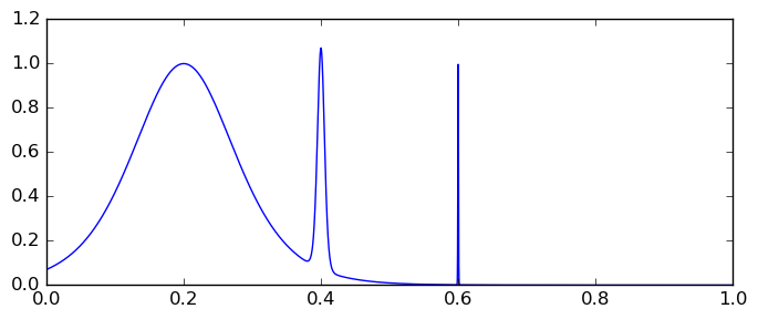
The acb.integral method wraps the rigorous numerical integration code in Arb.
Here is the infamous "spike integral" as an example: $$\int_0^1 \operatorname{sech}^2(10(x-0.2)) + \operatorname{sech}^4(100(x-0.4)) + \operatorname{sech}^6(1000(x-0.6)) dx = 0.2108027355\ldots$$
SciPy's quad gives an answer that is only accurate to two digits, although the error estimate suggests eight correct digits!
>>> from scipy.integrate import quad
>>> from scipy import cosh
>>> f = lambda x: cosh(10*x-2)**-2 + cosh(100*x-40)**-4 + cosh(1000*x-600)**-6
>>> quad(f, 0, 1)
(0.20973606883387982, 3.028145707813807e-09)
mpmath is just as inaccurate:
>>> from mpmath import quad, sech
>>> f = lambda x: sech(10*x-2)**2 + sech(100*x-40)**4 + sech(1000*x-600)**6
>>> quad(f, [0, 1])
mpf('0.20981978444322463')
Arb has no trouble with this integral:
>>> f = lambda x, _: (10*x-2).sech()**2 + (100*x-40).sech()**4 + (1000*x-600).sech()**6
>>> acb.integral(f, 0, 1)
[0.21080273550055 +/- 4.44e-15]
>>> ctx.dps = 50
>>> acb.integral(f, 0, 1)
[0.2108027355005492773756432557057291543609091864368 +/- 7.54e-50]
Integration works with special functions in the integrand. Here is an integral of the gamma function on a vertical segment in the complex plane:
>>> ctx.dps = 30
>>> acb.integral(lambda x, _: x.gamma(), 1, 1+100j)
[0.15447964132004274469018853480 +/- 7.04e-30] + [1.15572734979092171791009318331 +/- 8.34e-30]j
Many other interesting examples of integrals can be found in the integrals.c program included with Arb. It is straightforward to try most of those examples with Python-FLINT.
An important caveat when using acb.integral: the object function supplied by the user takes two inputs, the actual argument to the integrand and a boolean flag. When the flag is set, the object function must verify that the integrand is analytic on the argument. This is automatic for meromorphic functions (including the examples shown above), but for integrands with step discontinuities or branch cuts in the complex plane, the user must handle this flag manually! Some acb methods implementing functions with branch cuts support an optional keyword argument analytic, in which case the user can simply pass the flag through. The sqrt method is an example:
>>> ctx.dps = 50
>>> acb.integral(lambda x, _: 2 * (1-x**2).sqrt(), -1, 1)    # WRONG !!!
[3.2659863237109041309297120996078551892879299742089 +/- 1.70e-50] + [+/- 2.34e-59]j

>>> acb.integral(lambda x, a: 2 * (1-x**2).sqrt(analytic=a), -1, 1)     # correct
[3.14159265358979323846264338327950288419716939937 +/- 5.67e-48] + [+/- 1.34e-51]j
By the way, for a slightly more aesthetically pleasing output, acb.real_sqrt knows that the integrand is supposed to be purely real, so the imaginary part noise disappears:
>>> acb.integral(lambda x, a: 2 * (1-x**2).real_sqrt(analytic=a), -1, 1)
[3.14159265358979323846264338327950288419716939937 +/- 5.67e-48]
Roots of polynomials
Python-FLINT now makes it easy to compute all the roots (with multiplicities) of polynomials with integer or rational coefficients:
>>> x = fmpz_poly([0,1])
>>> f = ((3*x+5)*(1+x**3))**10 * (1-x**2) * (1-x+3*x**2-x**3)
>>> for c in f.roots():
...     print(c)
...
([1.00000000000000 +/- 9e-19], 1)
([2.76929235423863 +/- 1.42e-15], 1)
([0.115353822880684 +/- 2.94e-16] + [0.589742805022206 +/- 5.00e-16]j, 1)
([0.115353822880684 +/- 2.94e-16] + [-0.589742805022206 +/- 5.00e-16]j, 1)
([-1.66666666666667 +/- 3.34e-15], 10)
([0.500000000000000 +/- 4.0e-19] + [0.866025403784439 +/- 3.54e-16]j, 10)
([0.500000000000000 +/- 4.0e-19] + [-0.866025403784439 +/- 3.54e-16]j, 10)
(-1.00000000000000, 11)
It is also possible to compute the exact factorization of such a polynomial:
>>> f.factor()
(1, [(x + (-1), 1), (x^3 + (-3)*x^2 + x + (-1), 1), (3*x + 5, 10), (x^2 + (-1)*x + 1, 10), (x + 1, 11)])
For integer and rational polynomials, .roots() automatically computes the correct multiplicity of each root, separates all real roots from non-real roots (the imaginary parts in the output are either exactly zero or strictly nonzero), and computes all the roots to the full accuracy of the current working precision. The algorithm also scales reasonably well: it takes two seconds to find the roots of the Legendre polynomial of degree 200:
>>> fmpq_poly.legendre_p(200).roots()
[([-0.999928071285070 +/- 2.30e-17], 1),   ...   ([0.999928071285070 +/- 2.30e-17], 1)]
(This works with any polynomial, but it should be pointed out that Arb also has fast special-purpose code for roots of Legendre polynomials. This functionality is available as a method of the arb type:
>>> arb.legendre_p_root(200,0)
[0.999928071285070 +/- 2.26e-16]
>>> arb.legendre_p_root(200,1)
[0.999621031280936 +/- 4.90e-16]
>>> arb.legendre_p_root(200,199)
[-0.999928071285070 +/- 2.26e-16]
With this function, computing all the roots of $P_{200}(x)$ to 15-digit accuracy takes only 0.003 seconds. Optionally the Gauss-Legendre quadrature weights can also be computed.)
Root-finding also works for polynomials with inexact real or complex coefficients, but not in full generality (for example, multiple roots are not supported).
LLL-reducing matrices
Python-FLINT now exposes FLINT's implementation of the LLL algorithm for finding short lattice vectors. One of many possible applications is to search for integer relations between real numbers. As an example, take the following set of real numbers: $\pi/4, \sqrt{2}, \operatorname{atan}(1/5), \log(2), \operatorname{atan}(1/239)$.
>>> V = [arb.pi()/4, arb(2).sqrt(), (1/arb(5)).atan(), arb(2).log(), (1/arb(239)).atan()]
>>> n = len(V)
>>> A = fmpz_mat(n, n+1)
>>> for i in range(n):
...     A[i,i] = 1
...     A[i,n] = (V[i] * 2**(ctx.prec // 2)).floor().unique_fmpz()
...
>>> A.lll()
[   1,    0,   -4,    0,    1,     1]
[-109,  574, -227, -981, -326,  -473]
[-309,   16,  169,  262, 1218,  -229]
[-411,  121, -435,  342,  117, -1440]
[1200, -467,  -60, -388, -300, -1135]
The first row gives us Machin's formula $\pi/4 - 4 \operatorname{atan}(1/5) + \operatorname{atan}(1/239) = 0$. Exercise for the reader: turn this example into a function for finding integer relations in vectors of complex numbers, and add some more options!
Arbitrary-precision FFTs
A nice feature implemented in Arb by Pascal Molin and now exposed in Python-FLINT is support for computing arbitrary-precision discrete Fourier transforms (DFTs). The computation is done using FFT algorithms with $O(n \log n)$ complexity even for non-power-of-two sizes (although power-of-two sizes are more efficient). Here is an example of computing a DFT of length 12345 with 100-digit precision, and then inverting it:
>>> ctx.dps = 100
>>> v = acb.dft(range(12345))
>>> w = acb.dft(v, inverse=True)
>>> w[0]; w[1]; w[2]; w[-1]
[+/- 2.46e-85] + [+/- 2.46e-85]j
[1.000000000000000000000000000000000000000000000000000000000000000000000000000000000000 +/- 7.67e-85] + [+/- 7.67e-85]j
[2.000000000000000000000000000000000000000000000000000000000000000000000000000000000000 +/- 6.66e-85] + [+/- 6.66e-85]j
[12344.00000000000000000000000000000000000000000000000000000000000000000000000000000000000 +/- 1.96e-84] + [+/- 1.96e-84]j
>>> sum(w)
[76193340.0000000000000000000000000000000000000000000000000000000000000000000000000000000 +/- 1.72e-80] + [+/- 1.72e-80]j
In this example, each transform takes 0.4 seconds on my laptop.
How to print things?
The API is still a bit experimental, and there will certainly be compatibility-breaking changes in the next release. I hope to receive user feedback so that necessary breaking changes can be implemented sooner rather than later. One issue I would like immediate feedback about is whether pretty-printing should be enabled by default, and what the non-pretty-printed format should be. Right now, pretty-printing is the default:
>>> fmpq(-3)/2
-3/2
>>> ctx.pretty = False
>>> fmpq(-3)/2
fmpq(-3,2)
Non-pretty-printing has some advantages: it's nice to see the type of the output, and the result can be copied and pasted back in the REPL. However, I found that the verbose output quickly became tedious to look at, especially for matrices and lists of elements. An alternative might be to show the type constructor with readable string input:
>>> fmpq(-3,2)
fmpq("-3/2")
However, it still gets verbose when printing a Python list, for example. Also, with Arb numbers, one has the problem that a binary-decimal-binary roundtrip loses a significant amount of precision; a binary-exact repr() format could be used, but this would be completely unreadable to humans.
fredrikj.net |
Blog index |
 RSS feed |
Follow me on Mastodon |
Become a sponsor
RSS feed |
Follow me on Mastodon |
Become a sponsor