fredrikj.net / blog /
Benchmarking exact DFT computation
September 14, 2020
The discrete Fourier transform (DFT) is a standard numerical benchmark. What about the DFT with exact numbers? This post will compare the performance of Calcium, Sage's QQbar (exact field of algebraic numbers), Sage's SymbolicRing, SymPy, and Mathematica. The benchmark problem will be to evaluate $\textbf{x} - \operatorname{DFT}^{-1}(\operatorname{DFT}(\textbf{x}))$ where $$ \operatorname{DFT}(\textbf{x})_n = \sum_{k=0}^{N-1} \omega^{-kn} x_k, \quad \operatorname{DFT}^{-1}(\textbf{x})_n = \frac{1}{N} \sum_{k=0}^{N-1} \omega^{kn} x_k, \quad \omega = e^{2 \pi i / N}$$
for a few different input sequences $\mathbf{x} = (x_n)_{n=0}^{N-1}$. To make the benchmark meaningful, we require that $\textbf{x} - \operatorname{DFT}^{-1}(\operatorname{DFT}(\textbf{x}))$ simplifies to the zero vector. We thereby test the ability to contract (simplify) expressions and not just to expand. If a system fails to prove that some entry in the output vector is zero, it gets a (FAIL).
We test the following inputs: $x_n = n+2$, $x_n = \sqrt{n+2}$, $x_n = \log(n+2)$, $x_n = e^{2 \pi i / (n+2)}$, $x_n = \frac{1}{1+(n+2) \pi}$, and $x_n = \frac{1}{1+\sqrt{n+2} \pi}$, for lengths $N = 2,\ldots,20$ and $N = 30, 50, 100$ where reasonable.
Calcium example
This benchmark is implemented in the dft.c example program for Calcium. Here is a sample run with $N = 4$ and the sequence $x_n = \log(n+2)$:
fredrik@agm:~/src/calcium$ build/examples/dft 4 -verbose -input 2
DFT benchmark, length N = 4

[x] =
0.693147 {a where a = 0.693147 [Log(2)]}
1.09861 {a where a = 1.09861 [Log(3)]}
1.38629 {a where a = 1.38629 [Log(4)]}
1.60944 {a where a = 1.60944 [Log(5)]}

DFT([x]) =
4.78749 {a+c+3*d where a = 1.60944 [Log(5)], b = 1.38629 [Log(4)], c = 1.09861 [Log(3)], d = 0.693147 [Log(2)]}
-0.693147 + 0.510826*I {a*e-c*e-d where a = 1.60944 [Log(5)], b = 1.38629 [Log(4)], c = 1.09861 [Log(3)], d = 0.693147 [Log(2)], e = I [e^2+1=0]}
-0.628609 {-a-c+3*d where a = 1.60944 [Log(5)], b = 1.38629 [Log(4)], c = 1.09861 [Log(3)], d = 0.693147 [Log(2)]}
-0.693147 - 0.510826*I {-a*e+c*e-d where a = 1.60944 [Log(5)], b = 1.38629 [Log(4)], c = 1.09861 [Log(3)], d = 0.693147 [Log(2)], e = I [e^2+1=0]}

IDFT(DFT([x])) =
0.693147 {d where a = 1.60944 [Log(5)], b = 1.38629 [Log(4)], c = 1.09861 [Log(3)], d = 0.693147 [Log(2)], e = I [e^2+1=0]}
1.09861 {c where a = 1.60944 [Log(5)], b = 1.38629 [Log(4)], c = 1.09861 [Log(3)], d = 0.693147 [Log(2)], e = I [e^2+1=0]}
1.38629 {2*d where a = 1.60944 [Log(5)], b = 1.38629 [Log(4)], c = 1.09861 [Log(3)], d = 0.693147 [Log(2)], e = I [e^2+1=0]}
1.60944 {a where a = 1.60944 [Log(5)], b = 1.38629 [Log(4)], c = 1.09861 [Log(3)], d = 0.693147 [Log(2)], e = I [e^2+1=0]}

[x] - IDFT(DFT([x])) =
0       (= 0   T_TRUE)
0       (= 0   T_TRUE)
0       (= 0   T_TRUE)
0       (= 0   T_TRUE)

cpu/wall(s): 0.007 0.006
virt/peak/res/peak(MB): 36.28 36.28 8.75 8.75
A comment on the print format: 4.78749 {a+c+3*d where a = 1.60944 [Log(5)], b = 1.38629 [Log(4)], c = 1.09861 [Log(3)], d = 0.693147 [Log(2)]} means that the symbolic representation is $a+c+3d$ where $a = \log(5), c = \log(3), d = \log(2)$ and that the approximate numerical value is 4.78749.
The output of the inverse DFT is not exactly the same as the original vector $\mathbf{x}$, in terms of its symbolic representation: the fields of the coefficients have some "memory" of the other coefficients encountered in the computation, and $\log(4)$ has been transformed into $2 \log(2)$. Nevertheless, on subtraction of the two vectors, we get precisely zeros.
Benchmark implementation details
We evaluate the DFT by simple $O(N^2)$ summation. The purpose is to test symbolic arithmetic and simplification, and using an $O(N \log N)$ FFT algorithm does not matter much in this setting. We compute an array of roots of unity $1,\omega,\omega^2,\ldots,\omega^{2N-1}$ at the start for use in both the DFT and inverse DFT.
In Sage, SymPy and Mathematica, the result does not usually expand to 0 automatically, so we have to call .simplify_full(), FullSimplify[] or equivalent. In Calcium, it turns out that the result usually expands to 0 automatically, though in some cases we have to call ca_check_is_zero().
I don't have a copy of Mathematica (nor Maple), so for this benchmark I timed Mathematica on the free Wolfram Cloud which has a 1-minute timeout. I report (TIMEOUT) in cases where it did not finish. For other systems, I also report (TIMEOUT) where the computation did not finish in a few minutes. It should be noted that the hardware for the Wolfram Cloud is different from my own computer, so the absolute timings are not directly comparable (my CPU seems to be slower, but loads may vary). I used a single thread everywhere.
The systems cache various data, and as a result running the same code a second time can be much faster than the first time. For this benchmark, I have timed the first run (for each separate $N$) starting with an empty cache. In SymPy and Mathematica, this meant explicitly calling clear_cache() and ClearSystemCache[] at the start of the run. In Calcium, I include the time of setting up and destroying the context object.
I could have benchmarked the performance with a hot cache instead, but the data would not really be meaningful for cross-system comparison because different systems cache different kinds of information (theoretically, a system could cache the whole computation), and frankly it would have been too tedious to run the separate computations for all the systems and present the data. The downside is that Calcium looks worse than it should for small $N$, since in practice you'd often want to recycle the same context object for many calculations.
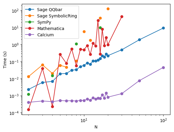
Test A: $x_n = n+2$
All timings are in seconds.
| N | Sage QQBar | Sage SymbolicRing | SymPy | Mathematica | Calcium |
| 2 | 0.0023 | 0.013 | 0.0012 | 0.00015 | 0.00040 |
| 3 | 0.0059 | 0.063 | (FAIL) | 0.039 | 0.00048 |
| 4 | 0.0068 | 0.020 | 0.015 | 0.00023 | 0.00044 |
| 5 | 0.019 | 0.060 | (FAIL) | 0.26 | 0.00051 |
| 6 | 0.020 | 0.047 | (FAIL) | 0.078 | 0.00049 |
| 7 | 0.031 | (FAIL) | (FAIL) | 0.55 | 0.00050 |
| 8 | 0.033 | 0.11 | 1.1 | 0.057 | 0.00048 |
| 9 | 0.050 | (FAIL) | (FAIL) | 0.52 | 0.00052 |
| 10 | 0.060 | 5.7 | (FAIL) | 0.49 | 0.00052 |
| 11 | 0.081 | (FAIL) | (FAIL) | 0.87 | 0.00062 |
| 12 | 0.069 | 1.8 | (FAIL) | 0.26 | 0.00053 |
| 13 | 0.11 | (FAIL) | (FAIL) | 1.2 | 0.00075 |
| 14 | 0.11 | (FAIL) | (FAIL) | 0.82 | 0.00062 |
| 15 | 0.12 | (FAIL) | (FAIL) | 26 | 0.00071 |
| 16 | 0.15 | 36 | 9.9 | 0.27 | 0.00068 |
| 17 | 0.22 | (FAIL) | (FAIL) | 7.9 | 0.0011 |
| 18 | 0.18 | (FAIL) | (FAIL) | 0.84 | 0.00071 |
| 19 | 0.27 | (FAIL) | (FAIL) | 2.6 | 0.0014 |
| 20 | 0.22 | 124 | (FAIL) | 0.96 | 0.00081 |
| 30 | 0.49 | (FAIL) | (FAIL) | 44 | 0.0013 |
| 50 | 1.9 | (FAIL) | (FAIL) | (TIMEOUT) | 0.0076 |
| 100 | 9.2 | (FAIL) | (FAIL) | (TIMEOUT) | 0.045 |
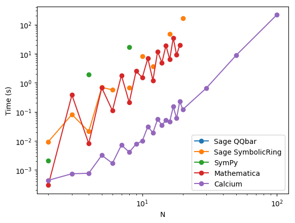
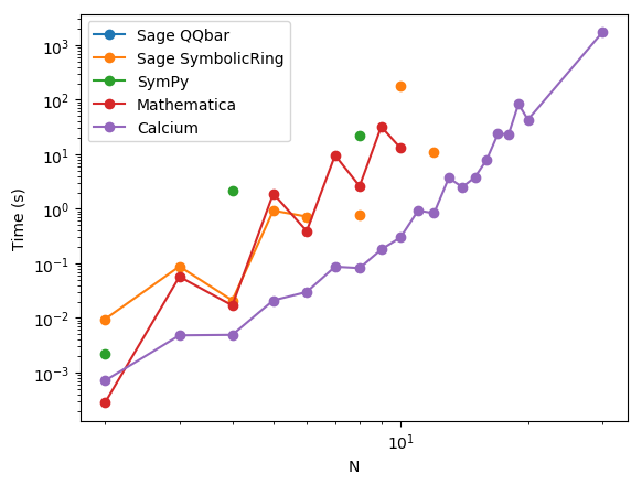
Comment: this is effectively a test of arithmetic in the cyclotomic field $\mathbb{Q}(\omega)$. I'm actually surprised that Sage's QQbar performs so poorly, because it is supposedly optimized for arithmetic in absolute number fields. Sage's SymbolicRing fails to simplify the result when $N$ has too many or large divisors, and SymPy only succeeds when $N$ is a power of two (this will be the case in all the other tests as well). For small $N$, Calcium's timings mostly show the overhead of precomputations: for example, if the context object were reused, $N = 4$ would take 0.000017 seconds (24 times faster). Anyway, Calcium is the clear champion when $N$ grows.
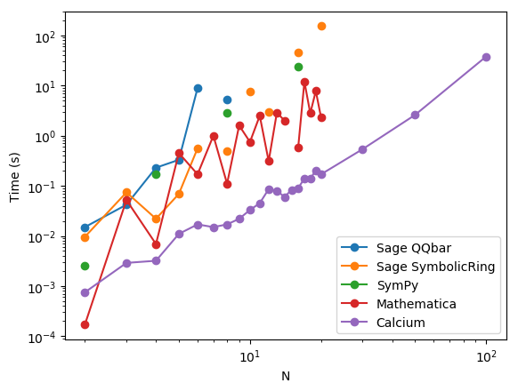
Test B: $x_n = \sqrt{n+2}$
| N | Sage QQBar | Sage SymbolicRing | SymPy | Mathematica | Calcium |
| 2 | 0.015 | 0.0096 | 0.0025 | 0.00017 | 0.00075 |
| 3 | 0.042 | 0.074 | (FAIL) | 0.052 | 0.0029 |
| 4 | 0.23 | 0.022 | 0.17 | 0.0069 | 0.0032 |
| 5 | 0.33 | 0.069 | (FAIL) | 0.45 | 0.011 |
| 6 | 8.9 | 0.56 | (FAIL) | 0.17 | 0.017 |
| 7 | (TIMEOUT) | (FAIL) | (FAIL) | 1.0 | 0.015 |
| 8 | 5.3 | 0.50 | 2.8 | 0.11 | 0.017 |
| 9 | (TIMEOUT) | (FAIL) | (FAIL) | 1.6 | 0.022 |
| 10 | (TIMEOUT) | 7.5 | (FAIL) | 0.75 | 0.033 |
| 11 | (TIMEOUT) | (FAIL) | (FAIL) | 2.5 | 0.045 |
| 12 | (TIMEOUT) | 3.0 | (FAIL) | 0.31 | 0.086 |
| 13 | (TIMEOUT) | (FAIL) | (FAIL) | 2.9 | 0.080 |
| 14 | (TIMEOUT) | (FAIL) | (FAIL) | 2.0 | 0.060 |
| 15 | (TIMEOUT) | (FAIL) | (FAIL) | (TIMEOUT) | 0.083 |
| 16 | (TIMEOUT) | 46 | 24 | 0.58 | 0.090 |
| 17 | (TIMEOUT) | (FAIL) | (FAIL) | 12 | 0.14 |
| 18 | (TIMEOUT) | (FAIL) | (FAIL) | 2.8 | 0.14 |
| 19 | (TIMEOUT) | (FAIL) | (FAIL) | 7.8 | 0.20 |
| 20 | (TIMEOUT) | 154 | (FAIL) | 2.3 | 0.17 |
| 30 | (TIMEOUT) | (FAIL) | (FAIL) | (TIMEOUT) | 0.54 |
| 50 | (TIMEOUT) | (FAIL) | (FAIL) | (TIMEOUT) | 2.6 |
| 100 | (TIMEOUT) | (FAIL) | (FAIL) | (TIMEOUT) | 38 |
Comment: this is effectively a test of multivariate algebraic number fields. It's also where Sage's QQBar starts to show its big weakness: since it only uses absolute fields internally for simplification, it becomes completely useless as soon as you mix different algebraic numbers that don't fit neatly into an absolute field. Other than that, the picture is similar to the previous: Sage's SymbolicRing and SymPy do a decent job for the few $N$ where they work, Mathematica runs just fine (although $N = 15$ takes over a minute for some reason), and Calcium handles everything easily.
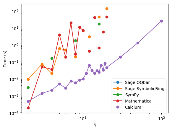
Test C: $x_n = \log(n+2)$
| N | Sage QQBar | Sage SymbolicRing | SymPy | Mathematica | Calcium |
| 2 | - | 0.0094 | 0.0031 | 0.00019 | 0.00047 |
| 3 | - | 0.073 | (FAIL) | 0.051 | 0.0014 |
| 4 | - | 0.021 | 0.16 | 0.036 | 0.0021 |
| 5 | - | 0.60 | (FAIL) | 3.8 | 0.0050 |
| 6 | - | 0.51 | (FAIL) | 0.19 | 0.0028 |
| 7 | - | (FAIL) | (FAIL) | 20 | 0.0074 |
| 8 | - | 0.20 | 1.8 | 0.29 | 0.0059 |
| 9 | - | (FAIL) | (FAIL) | 11 | 0.0083 |
| 10 | - | 6.7 | (FAIL) | 7.2 | 0.010 |
| 11 | - | (FAIL) | (FAIL) | (TIMEOUT) | 0.021 |
| 12 | - | 3.0 | (FAIL) | 0.42 | 0.061 |
| 13 | - | (FAIL) | (FAIL) | (TIMEOUT) | 0.032 |
| 14 | - | (FAIL) | (FAIL) | 41 | 0.021 |
| 15 | - | (FAIL) | (FAIL) | (TIMEOUT) | 0.030 |
| 16 | - | 44 | 17 | 0.66 | 0.025 |
| 17 | - | (FAIL) | (FAIL) | (TIMEOUT) | 0.061 |
| 18 | - | (FAIL) | (FAIL) | 5.9 | 0.033 |
| 19 | - | (FAIL) | (FAIL) | (TIMEOUT) | 0.082 |
| 20 | - | 136 | (FAIL) | 45 | 0.046 |
| 30 | - | (FAIL) | (FAIL) | (TIMEOUT) | 0.19 |
| 50 | - | (FAIL) | (FAIL) | (TIMEOUT) | 1.3 |
| 100 | - | (FAIL) | (FAIL) | (TIMEOUT) | 26 |
Comment: similar to the previous but with transcendental numbers instead of algebraic numbers. Obviously, Sage's QQbar is no longer applicable. Mathematica struggles a bit here, perhaps because of relations between the logarithms.
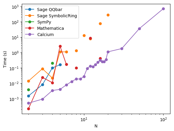
Test D: $x_n = e^{2 \pi i / (n+2)}$
| N | Sage QQBar | Sage SymbolicRing | SymPy | Mathematica | Calcium |
| 2 | 0.0015 | 0.014 | 0.0038 | 0.00022 | 0.00051 |
| 3 | 0.0081 | 0.088 | (FAIL) | 0.024 | 0.00093 |
| 4 | 0.10 | 0.022 | 0.20 | 0.011 | 0.0034 |
| 5 | 0.16 | 1.1 | (FAIL) | 2.6 | 0.0040 |
| 6 | (TIMEOUT) | 1.1 | (FAIL) | 0.17 | 0.0078 |
| 7 | (TIMEOUT) | (FAIL) | (FAIL) | (TIMEOUT) | 0.013 |
| 8 | (TIMEOUT) | 1.3 | (FAIL) | 0.10 | 0.019 |
| 9 | (TIMEOUT) | (FAIL) | (FAIL) | (TIMEOUT) | 0.019 |
| 10 | (TIMEOUT) | 13 | (FAIL) | (TIMEOUT) | 0.028 |
| 11 | (TIMEOUT) | (FAIL) | (FAIL) | (TIMEOUT) | 0.093 |
| 12 | (TIMEOUT) | 7.9 | (FAIL) | 8.7 | 0.13 |
| 13 | (TIMEOUT) | (FAIL) | (FAIL) | (TIMEOUT) | 0.12 |
| 14 | (TIMEOUT) | (FAIL) | (FAIL) | (TIMEOUT) | 0.16 |
| 15 | (TIMEOUT) | (FAIL) | (FAIL) | (TIMEOUT) | 0.23 |
| 16 | (TIMEOUT) | 78 | (TIMEOUT) | 0.41 | 0.32 |
| 17 | (TIMEOUT) | (FAIL) | (FAIL) | (TIMEOUT) | 0.26 |
| 18 | (TIMEOUT) | (FAIL) | (FAIL) | (TIMEOUT) | 0.26 |
| 19 | (TIMEOUT) | (FAIL) | (FAIL) | (TIMEOUT) | 0.35 |
| 20 | (TIMEOUT) | 277 | (FAIL) | (TIMEOUT) | 1.1 |
| 30 | (TIMEOUT) | (FAIL) | (FAIL) | (TIMEOUT) | 1.8 |
| 50 | (TIMEOUT) | (FAIL) | (FAIL) | (TIMEOUT) | 36 |
| 100 | (TIMEOUT) | (FAIL) | (FAIL) | (TIMEOUT) | 699 |
Comment: not enough roots of unity in the DFT to make things interesting? Then throw in more roots of unity :-) At $N = 100$ Calcium finished just when I was about to hit CTRL+C.
Test E: $x_n = 1/(1+(n+2)\pi)$
| N | Sage QQBar | Sage SymbolicRing | SymPy | Mathematica | Calcium |
| 2 | - | 0.0093 | 0.0021 | 0.00030 | 0.00044 |
| 3 | - | 0.081 | (FAIL) | 0.38 | 0.00074 |
| 4 | - | 0.021 | 1.9 | 0.0081 | 0.00077 |
| 5 | - | 0.69 | (FAIL) | 0.67 | 0.0032 |
| 6 | - | 0.57 | (FAIL) | 0.11 | 0.0017 |
| 7 | - | (FAIL) | (FAIL) | 1.8 | 0.0072 |
| 8 | - | 0.68 | 17 | 0.21 | 0.0041 |
| 9 | - | (FAIL) | (FAIL) | 2.5 | 0.0078 |
| 10 | - | 8.0 | (FAIL) | 1.5 | 0.0099 |
| 11 | - | (FAIL) | (FAIL) | 6.9 | 0.031 |
| 12 | - | 3.7 | (FAIL) | 1.2 | 0.019 |
| 13 | - | (FAIL) | (FAIL) | 11.9 | 0.056 |
| 14 | - | (FAIL) | (FAIL) | 4.9 | 0.035 |
| 15 | - | (FAIL) | (FAIL) | 19 | 0.051 |
| 16 | - | 48 | (TIMEOUT) | 6.4 | 0.046 |
| 17 | - | (FAIL) | (FAIL) | 35 | 0.15 |
| 18 | - | (FAIL) | (FAIL) | 9.0 | 0.06 |
| 19 | - | (FAIL) | (FAIL) | 20 | 0.23 |
| 20 | - | 167 | (FAIL) | (TIMEOUT) | 0.12 |
| 30 | - | (FAIL) | (FAIL) | (TIMEOUT) | 0.66 |
| 50 | - | (FAIL) | (FAIL) | (TIMEOUT) | 8.9 |
| 100 | - | (FAIL) | (FAIL) | (TIMEOUT) | 216 |
Comment: throwing in a denominator so that we exercise rational function arithmetic.
Test F: $x_n = \frac{1}{1+\sqrt{n+2} \pi}$
| N | Sage QQBar | Sage SymbolicRing | SymPy | Mathematica | Calcium |
| 2 | - | 0.0095 | 0.0022 | 0.00028 | 0.00071 |
| 3 | - | 0.088 | (FAIL) | 0.057 | 0.0048 |
| 4 | - | 0.021 | 2.19 | 0.017 | 0.0049 |
| 5 | - | 0.93 | (FAIL) | 1.9 | 0.021 |
| 6 | - | 0.72 | (FAIL) | 0.39 | 0.030 |
| 7 | - | (FAIL) | (FAIL) | 9.6 | 0.087 |
| 8 | - | 0.76 | 22 | 2.6 | 0.082 |
| 9 | - | (FAIL) | (FAIL) | 32 | 0.18 |
| 10 | - | 178 | (FAIL) | 13 | 0.30 |
| 11 | - | (FAIL) | (FAIL) | (TIMEOUT) | 0.93 |
| 12 | - | 11 | (FAIL) | (TIMEOUT) | 0.83 |
| 13 | - | (FAIL) | (FAIL) | (TIMEOUT) | 3.7 |
| 14 | - | (FAIL) | (FAIL) | (TIMEOUT) | 2.5 |
| 15 | - | (FAIL) | (FAIL) | (TIMEOUT) | 3.8 |
| 16 | - | (TIMEOUT) | (TIMEOUT) | (TIMEOUT) | 8.1 |
| 17 | - | (FAIL) | (FAIL) | (TIMEOUT) | 24 |
| 18 | - | (FAIL) | (FAIL) | (TIMEOUT) | 23 |
| 19 | - | (FAIL) | (FAIL) | (TIMEOUT) | 84 |
| 20 | - | (FAIL) | (FAIL) | (TIMEOUT) | 43 |
| 30 | - | (FAIL) | (FAIL) | (TIMEOUT) | 1720 |
| 50 | - | (FAIL) | (FAIL) | (TIMEOUT) | (TIMEOUT) |
| 100 | - | (FAIL) | (FAIL) | (TIMEOUT) | (TIMEOUT) |
Comment: similar to the previous example, except that the rational functions involve several variables.
Conclusion
Calcium turns out to do very well on this benchmark. I'm pleasantly surprised, because I expected that I'd have to do a lot more tweaking to even get it to work. I think to some extent this validates the design of Calcium. The usual disclaimer applies: Calcium is experimental, and future versions could be slower or faster. Notably, for small $N$, the performance from a cold start can still be improved; it's not really that important because most of the time you will want to reuse a context object, but it's a question of aesthetics :-)
Appendix: benchmarking code snippets
Thanks to Guillaume Moroz for the following Maple implementation:
idftdft := proc(coefficients)
    local N, unityroots, dft, idft, zeroes, result;
    N := nops(coefficients);
    unityroots := [seq(exp(I*2*Pi*k/N), k in 0..N-1)];
    dft := [ seq( add(coefficients[1+k]*unityroots[1+(k*n mod N)],
                      k in 0..N-1),
                  n in 0..N-1) ];
    idft := [ seq( add(dft[1+k]*unityroots[1+(-k*n mod N)],
                      k in 0..N-1)/N,
                  n in 0..N-1) ];
    zeroes := map(simplify, coefficients - idft):
    result := andmap(`=`, zeroes, 0);
    printnonzero(zeroes);
    return result;
end proc:

printnonzero := proc(L)
    local k;
    if not andmap(`=`, L, 0) then
        for k from 1 to nops(L) do
            if not evalb(L[k] = 0) then
                print(k, L[k]);
            end if;
        end do;
    end if;
end proc:

bench := proc(f, N)
    local coefficients, st, check, timing;
    forget(..); # Does not clear enough cache data
    lprint(f, N);
    coefficients := [seq(f(n), n in 0..N-1)];
    st := time():
    check := idftdft(coefficients);
    timing := time() - st;
    lprint(check);
    printf("%.3f\n\n",timing);
end proc:

bench(n -> n+2, 6):
bench(n -> n+2, 8):
bench(n -> n+2, 16):
bench(n -> n+2, 20):
bench(n -> n+2, 100):

#bench(n -> sqrt(n+2), 6):
#bench(n -> sqrt(n+2), 8):
#bench(n -> sqrt(n+2), 16):
#bench(n -> sqrt(n+2), 20):
#bench(n -> sqrt(n+2), 100): # long

#bench(n -> log(n+2), 6):
#bench(n -> log(n+2), 8):
#bench(n -> log(n+2), 16):
#bench(n -> log(n+2), 20):
#bench(n -> log(n+2), 100): # long

#bench(n -> exp(2*Pi*I/(n+2)), 6):
#bench(n -> exp(2*Pi*I/(n+2)), 8):
#bench(n -> exp(2*Pi*I/(n+2)), 16):
#bench(n -> exp(2*Pi*I/(n+2)), 20):
#bench(n -> exp(2*Pi*I/(n+2)), 100): # long

#bench(n -> 1/(1-(n+2)*Pi), 6):
#bench(n -> 1/(1-(n+2)*Pi), 8):
#bench(n -> 1/(1-(n+2)*Pi), 16):
#bench(n -> 1/(1-(n+2)*Pi), 20):
#bench(n -> 1/(1-(n+2)*Pi), 100): # long

#bench(n -> 1/(1+sqrt(n+2)*Pi), 6):
#bench(n -> 1/(1+sqrt(n+2)*Pi), 8):
#bench(n -> 1/(1+sqrt(n+2)*Pi), 16): # long
#bench(n -> 1/(1+sqrt(n+2)*Pi), 20):
#bench(n -> 1/(1+sqrt(n+2)*Pi), 100):
Mathematica:
check[NNN_] := Module[{NN = NNN},
ClearSystemCache[];
xs = Table[i+2, {i, 0, NN-1}];
ws = Table[Exp[2 Pi I k / NN], {k, 0, 2 NN - 1}];
ys = Table[Sum[xs[[k+1]]* ws[[1+Mod[-k*n, 2 NN]]], {k, 0, NN-1}], {n, 0, NN - 1}];
xs2 = Table[FullSimplify[Sum[ys[[k+1]]* ws[[1+Mod[k*n, 2 NN]]], {k, 0, NN-1}] / NN == xs[[n+1]]], {n, 0, NN - 1}]];
n=11; reps=1; {n, Timing[Do[check[n],{i,1,reps}]][[1]]/reps}
Comment: Daniel Schultz suggested using omega = ToNumberField[(-1)^(2/NN)]; ws = omega^Range[0, 2*NN-1]; in Mathematica. This seems to help on test A (expectedly) while it slows down the others.
SymPy and SageMath:
def benchSymPy(N, which=0, verbose=False):
    if which == 0:
        x = [S(i+2) for i in range(N)]
    elif which == 1:
        x = [sqrt(i+2) for i in range(N)]
    elif which == 2:
        x = [log(i+2) for i in range(N)]
    elif which == 3:
        x = [exp(2*pi*I/(i+2)) for i in range(N)]
    elif which == 4:
        x = [1/(1+(i+1)*pi) for i in range(N)]
    elif which == 5:
        x = [1/(1+sqrt(i+1)*pi) for i in range(N)]
    w1 = exp(2*pi*I/N)
    w = [w1**i for i in range(2*N)]
    y = [S(0) for i in range(N)]
    z = [S(0) for i in range(N)]
    for k in range(N):
        for n in range(N):
            y[k] += x[n] * w[(-k * n) % (2*N)]
    for k in range(N):
        for n in range(N):
            z[k] += y[n] * w[(k * n) % (2*N)]
        z[k] /= N
        eq = simplify(z[k] - x[k])
        if eq != 0:
            print(eq)
            raise ValueError


def benchQQbar(N, which=0):
    if which == 0:
        x = [QQbar(i+2) for i in range(N)]
    elif which == 1:
        x = [QQbar(i+2).sqrt() for i in range(N)]
    elif which == 3:
        x = [QQbar.zeta(i+2) for i in range(N)]
    w1 = QQbar.zeta(N)
    w = [w1**i for i in range(2*N)]
    y = [QQbar(0) for i in range(N)]
    z = [QQbar(0) for i in range(N)]
    for k in range(N):
        for n in range(N):
            y[k] += x[n] * w[(-k * n) % (2*N)]
    for k in range(N):
        for n in range(N):
            z[k] += y[n] * w[(k * n) % (2*N)]
        z[k] /= N
        if z[k] - x[k] != 0:
            raise ValueError

def benchSR(N, which=0, verbose=False):
    if which == 0:
        x = [SR(i+2) for i in range(N)]
    elif which == 1:
        x = [SR(i+2).sqrt() for i in range(N)]
    elif which == 2:
        x = [SR(i+2).log() for i in range(N)]
    elif which == 3:
        x = [SR(exp(2*pi*I/(i+2))) for i in range(N)]
    elif which == 4:
        x = [SR(1/(1+(i+1)*pi)) for i in range(N)]
    elif which == 5:
        x = [SR(1/(1+sqrt(i+1)*pi)) for i in range(N)]
    w1 = SR(exp(2*pi*I/N))
    w = [w1**i for i in range(2*N)]
    y = [SR(0) for i in range(N)]
    z = [SR(0) for i in range(N)]
    for k in range(N):
        for n in range(N):
            y[k] += x[n] * w[(-k * n) % (2*N)]
    for k in range(N):
        for n in range(N):
            z[k] += y[n] * w[(k * n) % (2*N)]
        z[k] /= N
        eq = (z[k] - x[k]).full_simplify()
        if eq != 0:
            raise ValueError
fredrikj.net |
Blog index |
 RSS feed |
Follow me on Mastodon |
Become a sponsor
RSS feed |
Follow me on Mastodon |
Become a sponsor