Galerkin’s method in SymPy

February 4, 2009

I’m currently taking a PDE course, and for this reason I am trying to come terms with the Galerkin method. The Galerkin method is conceptually simple: one chooses a basis (for example polynomials up to degree q, or piecewise linear functions) and assumes that the solution can be approximated as a linear combination of the basis functions. One then chooses the coefficients so as to make the error orthogonal to all basis functions; this amounts to computing a sequence of integrals (the inner products determining orthogonality) and then solving a linear system of equations.

Doing the calculations by hand can get very messy. Fortunately, it is straightforward to implement the Galerkin method e.g. for an ODE IVP in SymPy and have the ugly parts done automatically. The following function implements the global Galerkin method on an interval [x0, x1], using polynomials up to degree q as the basis. It is assumed that the 0th degree basis function is fixed to the initial value.


from sympy import *
sum = __builtins__.sum

def galerkin(ode, x, x0, x1, u0, q):
    basis = [x**k for k in range(q+1)]
    # Coefficients for the basis monomials
    xi = [Symbol("xi_%i" % k) for k in range(q+1)]
    # Solution function ansatz
    u = u0 + sum(xi[k]*basis[k] for k in range(1,q+1))
    # Form system of linear equations
    equations = [integrate(ode(u)*basis[k], (x, x0, x1)) \
        for k in range(1,q+1)]
    coeffs = solve(equations, xi[1:])
    return u.subs(coeffs)

In general, the integrals can get very complex, if not unsolvable, and one must fall back to numerical methods. But for a simple problem, SymPy can calculate the integrals and the symbolic solution provides insight. Solving the standard problem u’ – u = 0 (with solution u(x) = exp(x)):


x = Symbol('x')
ode = lambda u: u.diff(x) - u
for q in range(1,6):
    pprint(galerkin(ode, x, 0, 1, 1, q))

This outputs:


1 + 3*x
              2
    8*x   10*x
1 + --- + -----
     11     11
               2       3
    30*x   45*x    35*x
1 + ---- + ----- + -----
     29     116     116
                  2        3        4
    1704*x   882*x    224*x    126*x
1 + ------ + ------ + ------ + ------
     1709     1709     1709     1709
                     2         3         4        5
    31745*x   15820*x    5460*x    1050*x    462*x
1 + ------- + -------- + ------- + ------- + ------
     31739     31739      31739     31739    31739

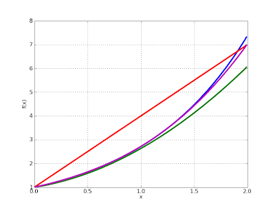
One can see that the coefficients rapidly approach those of Maclaurin polynomials for exp. The fast global convergence is also readily apparent upon visualization:


from mpmath import plot
u1 = Lambda(x, galerkin(ode, x, 0, 1, 1, 1))
u2 = Lambda(x, galerkin(ode, x, 0, 1, 1, 2))
u3 = Lambda(x, galerkin(ode, x, 0, 1, 1, 3))
plot([exp, u1, u2, u3], [0, 2])

The blue curve is exp(x). Note that the plotted interval is larger than the solution interval, so already the q = 3 solution (purple) is essentially accurate to within graphical tolerance. With moderately high degree, one gets a very accurate solution:


>>> galerkin(ode, x, 0, 1, 1, 10).subs(x,'7/10').evalf()
2.01375270747023
>>> exp('7/10').evalf()
2.01375270747048

The Galerkin method might prove useful as an alternative algorithm for high-precision ODE solving in mpmath. Mpmath has no problem with the nonlinear integrations, nor with solving the linear system in case it gets ill-conditioned at higher degree.

I’ll perhaps post some more code on this topic in the future, e.g. for solving the ODE with trigonometric and piecewise polynomial basis functions.

fredrikj.net | Blog index | RSS feed | Follow me on Mastodon | Become a sponsor