fredrikj.net / blog /
Massive hypergeometric update
June 19, 2009
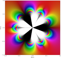
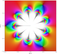
[Update: as further proof that the asymptotic expansions are working, I've plotted 1/erfi(1/z3), Ai(1/z3) and Bi(1/z3) around 0:
 |
 |
 |
End of update.]
Today I committed a large patch to mpmath that significantly improves the state of hypergeometric functions. It’s the result of about a week of work (plus some earlier research).
Perhaps most importantly, I’ve implemented the asymptotic expansions for 0F1 and 1F1 (the expansions for 2F1 were discussed in the previous post). They should now work for arbitrarily large arguments, as such:
>>> from mpmath import *
>>> mp.dps = 25
>>> print hyp0f1(3,100)
786255.7044208151250793134
>>> print hyp0f1(3,100000000)
4.375446848722142947128962e+8675
>>> print hyp0f1(3,10**50)
4.263410645749930620781402e+8685889638065036553022515
>>> print hyp0f1(3,-10**50)
-2.231890729584050840600415e-63
>>> print hyp0f1(1000,1000+10**8*j)
(-1.101783528465991973738237e+4700 - 1.520418042892352360143472e+4700j)
>>> print hyp1f1(2,3,10**10)
2.15550121570157969883678e+4342944809
>>> print hyp1f1(2,3,-10**10)
2.0e-20
>>> print hyp1f1(2,3,10**10*j)
(-9.750120502003974585202174e-11 - 1.746239245451213207369885e-10j)
I also implemented 2F0 and U (Kummer’s second function), mostly as a byproduct of the fact that 2F0 is needed for the asymptotic expansions of both 0F1 and 1F1. 2F0 is an interesting function: it is given by a divergent series (it converges only in special cases where it terminates after finitely many steps):
However, it can be assigned a finite value for all z by expressing it in terms of U. Hence, mpmath can now compute the regularized sum of 2F0(a,b,z) for any arguments, say these ones:
>>> print hyp2f0(5, -1.5, 4)
(0.0000005877300438912428637649737 + 89.51091139854661783977495j)
>>> print hyp2f0(5, -1.5, -4)
102.594435262256516621777
(This ought to be a novel feature; SciPy and GSL implement 2F0, but only special cases thereof, and Mathematica doesn’t have a direct way to evaluate 2F0.)
It’s the asymptotic case where z → 0, where a truncation of the 2F0 series can be used, that is used for the expansions at infinity of 0F1 and 1F1.
Back to 0F1 and 1F1, the asymptotic expansions of these functions are important because they permit many special functions to be evaluated efficiently for large arguments. So far I’ve fixed erf, erfc, erfi, airyai and airybi to take advantage of this fact (except for erf and erfc of a real variable, all these functions were previously slow even for a moderately large argument, say |z| > 100).
Examples that now work (well, some of them possibly theoretically worked before too, but probably required hours or ages of universe to finish):
>>> print erf(10000+10000j)
(1.000001659143196966967784 - 0.00003985971242709750831972313j)
>>> print erfi(1000000000)
2.526701758277367028229496e+434294481903251818
>>> print erfc(1000-5j)
(-1.27316023652348267063187e-434287 - 4.156805871732993710222905e-434288j)
>>> print airyai(10**10)
1.162235978298741779953693e-289529654602171
>>> print airybi(10**10)
1.369385787943539818688433e+289529654602165
>>> print airyai(-10**10)
0.0001736206448152818510510181
>>> print airybi(-10**10)
0.001775656141692932747610973
>>> print airyai(10**10 * (1+j))
(5.711508683721355528322567e-186339621747698 + 1.867245506962312577848166e-186339621747697j)
>>> print airybi(10**10 * (1+j))
(-6.559955931096196875845858e+186339621747689 - 6.822462726981357180929024e+186339621747690j)
An essential addition in this patch is the function hypercomb which evaluates a linear combination of hypergeometric series, with gamma function and power weights:
This is an extremely general function. Here is a partial list of functions that can be represented more or less directly by means of it:
- Regularized hypergeometric series
- The generalized incomplete gamma and beta functions (and their regularizations)
- Bessel functions
- Airy, Whittaker, Kelvin, Struve functions, etc
- Error functions
- Exponential, trigonometric and hyperbolic integrals
- Legendre, Chebyshev, Jacobi, Laguerre, Gegenbauer polynomials
- The Meijer G-function
That’s most of Abramowitz & Stegun, and means that the remaining hypergeometric-type functions available in Mathematica or Maxima but absent in mpmath will be easy to implement in the near future. With these additions, mpmath will have the most comprehensive support for numerical hypergeometric-type functions of any open source software, and should be very close to Mathematica.
The most important virtue of hypercomb is not that it allows for more concise implementations of various hypergeometric-type functions, although that is a big advantage too. The main idea is that hypercomb can deal with singular subexpressions, and particularly with gamma function poles that cancel against singularities in the hypergeometric series. These cases are almost more common than the nonsingular cases in practice, and hypercomb saves the trouble of handling them in every separate function.
Thus, in principle, a numerically correct implementation of hypercomb leads to correct implementations of all the functions in the list above. It’s not a silver bullet, of course. For example, if a particular but very common case of some common function triggers an expensive limit evaluation in hypercomb, then it’s probably better to handle that case with special-purpose code. There are also most likely some bugs left in hypercomb, although by now I have tested a rather large set of examples; large enough to be confident that it works soundly.
To show an example of how it works, an implementation of the Bessel J function might look like this:
def besj(n,z):
 z = mpmathify(z)
 h = lambda n: [([z/2],[n],[],[n+1],[],[n+1],-(z/2)**2)]
 return hypercomb(h, [n])

>>> mp.dps = 30
>>> print besselj(3,10.5)
0.1632801643733625756462387
>>> print besselj(-3,10.5)
-0.1632801643733625756462387
>>> print besj(3,10.5)
0.1632801643733625756462387
>>> print besj(-3,10.5)
-0.1632801643733625756462387
It gives the same value as the current Bessel J implementation in mpmath. Note that it works even when n is a negative integer, whereas naively evaluating the equation defining J(n,z) hits a gamma function pole and a division by zero in the hypergeometric series.
Thanks to the support for asymptotic expansions, this implementation (unlike the current besselj will also work happily with large arguments):
>>> print besj(3,1e9)
0.00000521042254280399021290721662036
I’m soon going to fix all the Bessel functions in mpmath along these lines, as I already did with erf, airyai, etc.
Here is another, more involved example (quoting directly from the docstring for hypercomb). The following evaluates
with a=1, z=3. There is a zero factor, two gamma function poles, and the 1F1 function is singular; all singularities cancel out to give a finite value:
>>> from mpmath import *
>>> mp.dps = 15
>>> print hypercomb(lambda a: [([a-1],[1],[a-3],[a-4],[a],[a-1],3)], [1])
-180.769832308689
>>> print -9*exp(3)
-180.769832308689
With some tweaks, the same code perhaps with a few tweaks could be used to symbolically evaluate hypergeometric-type functions (in the sense of rewriting them as pure hypergeometric series, and then possibly evaluating those symbolically as a second step). Symbolic support for hypergeometric functions is a very interesting (and hard) problem, and extremely important for computer algebra, but unfortunately I don’t have time to work on that at the moment (there is more than enough to do just on the numerical side).
fredrikj.net |
Blog index |
RSS feed |
Follow me on Mastodon |
Become a sponsor


