Meijer G, more hypergeometric functions, fractional differentiation

June 29, 2009

My last update and the post before it detailed substantial improvements to the code for hypergeometric functions in mpmath, specifically the support for asymptotic expansions for 0F1, 1F1, 2F1, 2F0, plus the ability to evaluate hypergeometric-type formulas with singular parameters.

Over the past week-and-a-half I’ve done more work along the same lines. Importantly, I’ve implemented asymptotic expansions also for 1F2, 2F2 and 2F3 (commits 1, 2), so all hypergeometric functions of degree up to (2,3) now support fast evaluation for |z| → ∞ (1F0 also works, if anyone wonders — it just happens to be a trivial case).

The next major remaining case is 3F2. It has a 1/z transformation, but this leaves |z| ≈ 1 which I don’t know how to deal with. Does anyone who happens to be reading this know methods for evaluating 3F2 close to the unit circle? Taylor expansion around some point other than 0 works to some extent, but it’s slow and in particular asymptotically slow close to z = 1, so not much help.

Bessel functions, etc.

As expected, the hypercomb function leads to very simple implementations of a large class of functions. I’ve now implemented the Whittaker, Struve, and Kelvin functions (they are called whitm, whitw, struveh, struvel, ber, bei, ker, kei). I’ve yet to update the orthogonal polynomials, but that shouldn’t be much work. With this, I will have covered most of Bessel-type and hypergeometric-type functions listed on the Wolfram Functions site.

Speaking of Bessel functions, I also addressed most of the problems with their implementation in this commit. In particular, they can now be evaluated for huge arguments:


>>> mp.dps = 30
>>> print besselj(1, 10**20)
-7.95068198242545016504555020084e-11
>>> print chop(besselj(1, 10**20 * j))
(0.0 + 5.17370851996688078482437428203e+43429448190325182754j)
>>> print bessely(1,10**20)
-6.69800904070342428527377044712e-12
>>> print besselk(1,10**20)
9.66424757155048856421325779143e-43429448190325182776

This wasn’t trivial, mainly because although hypercomb generally works, it sometimes becomes impossibly slow when computing functions straight from the definition. Basically: the function of interest might decrease exponentially, but internally it is computed by adding two nearly identical terms that grow exponentially, so the working precision and computation time increases exponentially. It’s therefore still necessary to switch between different representations in different parts of the complex plane, and figuring that out involves some work. Some cases probably remain to be fixed.

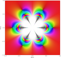
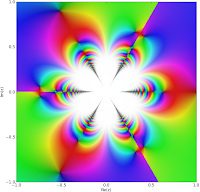
As a followup to last week, I’ll attach plots of J₀(1/z³), Y₀(1/z³) and K₀(1/z³):

The K plot unfortunately took very long time to finish — almost an hour for 200,000 complex evaluations (J and Y were both much faster), so I’ll probably have to optimize besselk a bit further.

Fractional derivatives

Another useful enhancement to the Bessel functions is that they can now be differentiated and integrated directly:


>>> mp.dps = 30
>>> print besselj(0, 3.5, derivative=2)
0.419378462090785430440501275011
>>> print diff(lambda x: besselj(0,x), 3.5, 2)
0.419378462090785430440501275011
>>> print besselj(0,3.5,derivative=-1) - besselj(0,2.5,derivative=-1)
-0.244675206320579138611991019242
>>> print quad(lambda x: besselj(0,x), [2.5, 3.5])
-0.244675206320579138611991019242

In fact, the representation for the derivatives works not just for integer orders (including negative values — giving iterated integrals), but also for fractional or complex values. This led me to implement a general function differint for computing fractional order derivatives / integrals of arbitrary functions. (Commit.) It works essentially directly with the definition of the Riemann-Liouville differintegral.

It gives the same result as the special-purpose implementation for the Bessel function:


>>> print besselj(0, 3.5, derivative=0.5)
-0.436609427860836504473775239357
>>> print differint(lambda x: besselj(0,x), 3.5, 0.5)
-0.436609427860836504473775239357

One neat application is iterated integration. The following gives a 5-fold integral of f(x) = exp(π x), along with the symbolic evaluation of the same as a check:


>>> print differint(lambda x: exp(pi*x), 3.5, -5, x0=-inf)
194.790546022218468869246881408
>>> print exp(pi*3.5) / pi**5
194.790546022218468869246881408

Does anyone have any other interesting applications for fractional differentiation? I’d be interested in more examples to test with and possibly add to the documentation.

The Meijer G-function

At last, the Meijer G-function is implemented! (Commit.) Personally, I think this is something of a milestone for the mpmath project.

The Meijer G-function is very important because of its role in symbolic definite integration. Basically, definite integrals of Meijer G-functions (and even products of Meijer G-functions) just yield new Meijer G-functions; Mathematica and Maple therefore do many integrals by rewriting the input in terms of Meijer G-functions, applying Meijer G transformations, and converting the result back to simpler functions if possible.

Having the Meijer G-function in mpmath should be useful for anyone who wishes to implement a more powerful definite integrator in SymPy for example. It could also be useful for obtaining numerical values from integrals done by hand.

Looking around for examples to do stress testing with, I found a web page by Viktor Toth: Maple and Meijer’s G-function: a numerical instability and a cure. His problem is to accurately evaluate G(-; 0; -1/2,-1,-3/2; -; x) for large real values of x. With my Meijer G-function implementation, I get:


>>> mp.dps = 15
>>> print meijerg([[],[0]],[[-0.5,-1,-1.5],[]],10)
4.89717497704114e-5
>>> print meijerg([[],[0]],[[-0.5,-1,-1.5],[]],100)
1.09696661341118e-12
>>> print meijerg([[],[0]],[[-0.5,-1,-1.5],[]],1000)
0.0
>>> print meijerg([[],[0]],[[-0.5,-1,-1.5],[]],10000)
1.53249554086589e+54

The third value should probably be small but not quite zero, and the last value is clearly bogus. Without looking at the details, the cause is almost certainly catastrophic cancellation of two huge terms. Fortunately, there is a cure for this:


>>> print meijerg([[],[0]],[[-0.5,-1,-1.5],[]],1000, check_cancellation=True)
3.34093555343418e-33
>>> print meijerg([[],[0]],[[-0.5,-1,-1.5],[]],10000, check_cancellation=True)
2.43925769071996e-94

The cancellation check should probably be enabled by default, either to automatically redo the computation as above or at least to issue a warning. The only catch with this is that it might lead to unnecessary slowdown and/or annoyance for the user in some cases, so I’ll have to investigate how common those cases are.

Incidentally, I also tried plugging the above two calculations into Mathematica 6.0. It takes a long time to finish (mpmath gives the result instantaneously) — and returns values that are wrong!


In[1]:= u1 = MeijerG[{{},{0}},{{-1/2,-1,-3/2},{}},1000]

                           3         1
Out[1]= MeijerG[{{}, {0}}, {{-(-), -1, -(-)}, {}}, 1000]
                           2         2

In[2]:= u2 = MeijerG[{{},{0}},{{-1/2,-1,-3/2},{}},10000]

                           3         1
Out[2]= MeijerG[{{}, {0}}, {{-(-), -1, -(-)}, {}}, 10000]
                           2         2

In[3]:= Timing[N[u1,20]]

Out[3]= {8.90265, 0.0017597930166135139087}

In[4]:= Timing[N[u1,50]]

                                                                    -33
Out[4]= {12.8231, 3.3409355534341801158987353523397047765918571151576 10   }

In[5]:=  Timing[N[u2,20]]

                                      50
Out[5]= {59.017, -2.0782671663885270791 10  }

In[6]:= Timing[N[u2,50]]

                                                                     22
Out[6]= {83.3753, -2.8700325450226332558088281915945389986057044454640 10  }

In[7]:= Timing[N[u2,120]]

Out[7]= {451.365, 2.439257690719956395903324691434088756714300374716395499173\

                                                                    -94
>      70196218529840153673260714339051464703903148052541923961351654 10   }

That’s several minutes for something mpmath did in less than a second, and with less intervention. So maybe Maple and Mathematica should copy my Meijer G-function code ;-)

Complex roots

A small and trivial, but quite convenient, new feature: the nthroot function can now compute any of the roots of a given number and not just the principal root. I also added root as an alias since I have lazy fingers. Like so:


>>> for k in range(5):
...     r = root(-12, 5, k)
...     print chop(r**5), r
...
-12.0 (1.32982316461435 + 0.966173083818997j)
-12.0 (-0.507947249855734 + 1.56330088863444j)
-12.0 -1.64375182951723
-12.0 (-0.507947249855734 - 1.56330088863444j)
-12.0 (1.32982316461435 - 0.966173083818997j)

While I was at it, I couldn’t resist also implementing a function unitroots for computing all the nth roots of unity, optionally just the primitive roots, as well as a function cyclotomic for evaluating the nth cyclotomic polynomial. As it turns out, cyclotomic polynomials are not entirely trivial to evaluate both efficiently and in a numerically stable way — see the source code for my solution. Commit here. A side effect is that I also implemented a powm1 function that accurately gives x^y – 1 (possibly a useful complement to expm1 for other uses as well):


>>> print power(2,1e-100)-1
0.0
>>> print powm1(2, 1e-100)
6.93147180559945e-101

That will be all for now.

fredrikj.net | Blog index | RSS feed | Follow me on Mastodon | Become a sponsor