Mpmath 0.14 released

February 5, 2010

I’ve just released version 0.14 of mpmath! Some highlights in this release have been covered in previous development updates on this blog:

mpmath in Sage to become 3x faster – a Cython extension module will be added to Sage that greatly speeds up mpmath (the Sage patch is currently being reviewed; if all goes to plan, the patch will be accepted soon and the mpmath version in Sage will be updated to 0.14 at the same time).
Zeta evaluation with the Riemann-Siegel expansion – Juan Arias de Reyna contributed code for very efficient and robust evaluation of the Riemann zeta function for arguments with large imaginary part.
Various features discussed in this update: 3D surface plotting (wrapping matplotlib, matrix calculus (transcendental functions of a matrix argument), Borel summation of divergent hypergeometric series, and options for whether to use Mathematica’s conventions for hypergeometric functions have been added.
Improved accuracy for hypergeometric functions with large parameters, and analytic continuation implemented for 3F2, 4F3, and higher hypergeometric functions.
Support for using Python floats/complexes for faster low-precision math. This is very handy for plotting, multidimensional integration, and other things requiring many function evaluations.

There are many other changes as well. See the CHANGES file and the list of commits for more details. Thanks to Juan Arias de Reyna, Vinzent Steinberg, Jorn Baayen and Chris Smith who contributed patches, and various people who tested and submitted bug reports (thanks also to anyone else I forgot to mention).

I’m sorry that it took several months to finish this release! This was partly due to large internal reorganizations done in order to support floats and the Cython backend in Sage. I’ve also had to take some time off to focus on my studies and other things.

An example: spherical harmonics

Here I will demonstrate three new features with a single example: 3D plotting, one of the newly added special functions (spherical harmonics), and low-precision evaluation with the fp context. Of course, everything here can be done in arbitrary precision with mp as well; fp is just faster for plotting.

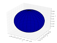
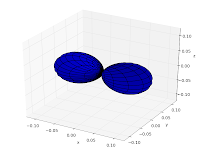
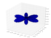
The following code visualizes spherical harmonics using a 3D polar plot. I’ve chosen to visualize the real part; the code is easily edited to show the absolute value (for example) instead.

from mpmath import fp
def Y(m,n):
def g(theta,phi):
R = fp.re(fp.spherharm(m,n,theta,phi))**2
x = R*fp.cos(phi)*fp.sin(theta)
y = R*fp.sin(phi)*fp.sin(theta)
z = R*fp.cos(theta)
return [x,y,z]
return g

fp.splot(Y(0,0), [0,fp.pi], [0,2*fp.pi])

The first few spherical harmonics are thus:

Y(0,0)
Y(1,0)	Y(1,1)
Y(2,0)	Y(2,1)	Y(2,2)
Y(3,0)	Y(3,1)	Y(3,2)
		Y(3,3)

Some numerical examples

A selection of evaluations that were not implemented, failed, gave inaccurate results or were extremely slow in previous versions of mpmath:

>>> from mpmath import *
>>> mp.dps = 25; mp.pretty = True
# reflection formula for Barnes G-function
>>> barnesg(-100000+10000j)
(-7.332534002219787256775675e+22857579769 +
1.304469872717249495403882e+22857579770j)

# Riemann zeta function, large height
>>> zeta(0.5+100000000j)
(-3.362839487530727943146807 + 1.407234559646447885979583j)

# Accurate evaluation of large-degree Bernoulli polynomial
>>> bernpoly(1000,100)
4.360903799140670486890619e+1996

# Computation of Euler numbers
>>> eulernum(20)
370371188237525.0
>>> eulernum(50, exact=True)
-6053285248188621896314383785111649088103498225146815121L
>>> eulernum(2000000000000000000)
3.19651108713502662532039e+35341231273461153426

# Accurate evaluation of hypergeometric functions with large parameters
>>> hyp2f1(1000,50,25,-1)
-2.886992344761576738138864e-274
>>> legenp(0.5, 300, 0.25)
-1.717508549497252387888262e+578
>>> besseli(2, 10, derivative=100)
821.2386210064833486609255

# Evaluation of 4F3 and 4F2
>>> hyper([1,2.125,3.25,4.5], [5.25,6.5,7], 1+2j)
(1.006737556189825231039221 + 0.3058770612264986390003873j)
>>> hyper([1,2.125,3.25,4.5], [5.25,6.5], 1+2j)
(0.3220085070641791195103201 + 0.5251231752161637627314328j)

# Matrix functions
>>> A = matrix([[2,3,1+j],[1,0,-1],[2,1,5]])
>>> mnorm(A - logm(expm(A)))
9.540212722670391941827867e-25
>>> mnorm(A - expm(logm(A)))
4.375286550134565812513542e-26
>>> nprint(expm(2*A))
[ (-2855.4 + 10733.0j) (-1871.95 + 8597.9j) (-7721.42 + 12906.7j)]
[(-3910.68 - 1749.82j) (-3152.69 - 1272.11j) (-4460.18 - 3558.54j)]
[ (17039.0 + 22621.8j) (14320.3 + 17405.9j) (13587.7 + 35087.8j)]
>>> nprint(expm(A)**2)
[ (-2855.4 + 10733.0j) (-1871.95 + 8597.9j) (-7721.42 + 12906.7j)]
[(-3910.68 - 1749.82j) (-3152.69 - 1272.11j) (-4460.18 - 3558.54j)]
[ (17039.0 + 22621.8j) (14320.3 + 17405.9j) (13587.7 + 35087.8j)]
>>> nprint(chop(sqrtm(A)*sqrtm(A)))
[2.0 3.0 (1.0 + 1.0j)]
[1.0 0.0 -1.0]
[2.0 1.0 5.0]

# A convenience function for precise evaluation of exp(j*pi*x)
>>> expjpi(36); exp(j*pi*36)
(1.0 + 0.0j)
(1.0 + 4.702307256907087875509661e-25j)

# Some fp functions have specialized implementations
# for improved speed and accuracy
>>> fp.erfc(5); float(mp.erfc(5))
1.5374597944280347e-12
1.5374597944280349e-12
>>> fp.erf(5); float(mp.erf(5))
0.99999999999846256
0.99999999999846256
>>> fp.ei(-12-3j); complex(mp.ei(-12-3j))
(4.6085637890261843e-07-3.141592693919709j)
(4.6085637890261901e-07-3.141592693919709j)
>>> fp.zeta(-0.5); float(fp.zeta(-0.5)) # real-argument fp.zeta
-0.20788622497735468
-0.20788622497735468
>>> fp.ci(40); float(mp.ci(40))
0.019020007896208769
0.019020007896208765
>>> fp.gamma(4+5j); complex(mp.gamma(4+5j))
(0.14965532796078551+0.31460331072967695j)
(0.14965532796078521+0.31460331072967596j)

For more examples and images, see the posts linked at the top of this post!

fredrikj.net | Blog index | RSS feed | Follow me on Mastodon | Become a sponsor