fredrikj.net / blog /
Taking the error out of the error function
March 16, 2016
Implementing interval versions of standard mathematical functions for Arb is an iterative process. The first goal is always to write a version that is correct, meaning that it must compute an interval with a correct error bound no matter the input. Then come optimizations. There are two kinds of optimizations: improving evaluation speed, and tightening error bounds. The latter kind improves Arb's effective speed too, at least if the increase in cost for computing tighter error bounds is not too significant, since tighter bounds allow users to work with lower precision and/or fewer evaluation points.
To be useful, error bounds should at least be effectively continuous in the following sense: if $f$ is continuous at the point $x$, then for a family of inputs $[x \pm \delta]$ and working precision of $p$ bits, the result of evaluating $f([x \pm \delta])$ should be an interval $[f(x) \pm \varepsilon]$ where $\varepsilon \to 0$ when both $p \to \infty$ and $\delta \to 0$. This tells us that it will work well to evaluate the function at "point values" such as $x = 1/2$ (which is exact) or $x = 7/3 + \pi$ (which cannot be represented exactly, but which can be enclosed by as narrow an interval as we like).
An even stronger quality demand is that error bounds should be reasonably tight when the input consists of wide intervals, where we cannot make $\delta \to 0$, at least not quickly enough. This becomes a concern if we want to bound the range of a function on an interval, or locate its roots or extrema rigorously. If we want to bound a function on $[0,1]$, say, we could easily evaluate it on 100 subintervals of width $0.01$, but evaluating it on $2^p$ intervals of width $2^{-p}$ is not feasible if $p$ has to be increased linearly, because the running time then increases exponentially.
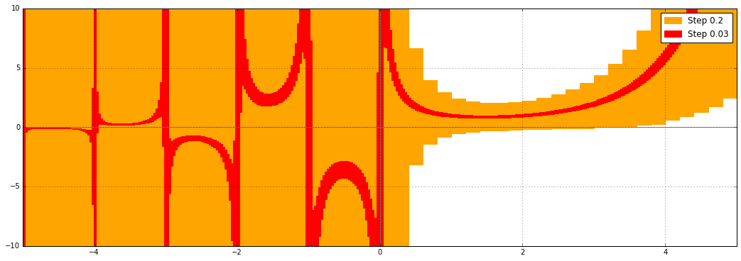
This is what the error function (erf) in Arb used to look like, when evaluated on wide intervals $[a, a+0.2]$ and slightly less wide intervals $[a, a+0.03]$, at 53-bit precision:
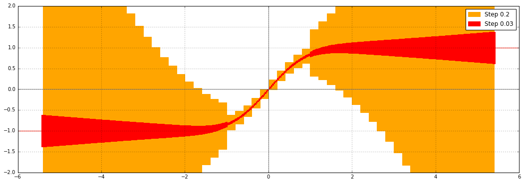
We see that the error bounds are converging when the input intervals get narrower, but the output intervals in the range of about $1 < |x| < 5.5$ are clearly very far from optimal. Why is this?
For real $|x| < 1$, the naive way to compute erf by the hypergeometric series $$\operatorname{erf}(x) = \frac{2x}{\sqrt{\pi}} {}_1F_1(\tfrac{1}{2}, \tfrac{3}{2}, -x^2)$$ works well, because the terms of the series decrease rapidly, so we are basically just perturbing the prefactor $2x /\sqrt{\pi}$ slightly. For $|x|$ greater than about 5.5, the asymptotic expansion $$\operatorname{erf}(x) = \frac{x}{\sqrt{x^2}} \left(1 - \frac{e^{-x^2}}{\sqrt{\pi}} U(\tfrac{1}{2}, \tfrac{1}{2}, x^2)\right)$$ kicks in at this precision, and we also get nice, tight error bounds.
For $|x| > 1$, and below the range of the asymptotic series, there would be catastrophic cancellation in the hypergeometric series, and the error bounds would blow up as $e^{x^2}$. In fact, Arb is slightly more clever. For $|x| > 1$ up to $|x| \approx 5.5$ (where the second point is dependent on the precision), Arb uses the formula $$\operatorname{erf}(x) = \frac{2x e^{-x^2}}{\sqrt{\pi}} {}_1F_1(1, \tfrac{3}{2}, x^2).$$ This avoids cancellation and therefore gives much better bounds than the first series, but there is still a problem: we are effectively computing two large exponentials and dividing them. In interval arithmetic, dividing two variables with dependent errors combines the errors instead of cancelling them out, and this is what causes the inflated bounds seen in the plot. The inflation is far less severe than it would be with the alternating series, but still far from optimal.
We can increase the working precision to compensate if $x$ is a point value (exact or as precise as the internal working precision needed to overcome cancellation), but this doesn't help when $x$ is a wide interval such as $[3.2, 3.4]$.
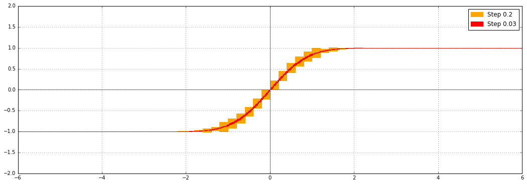
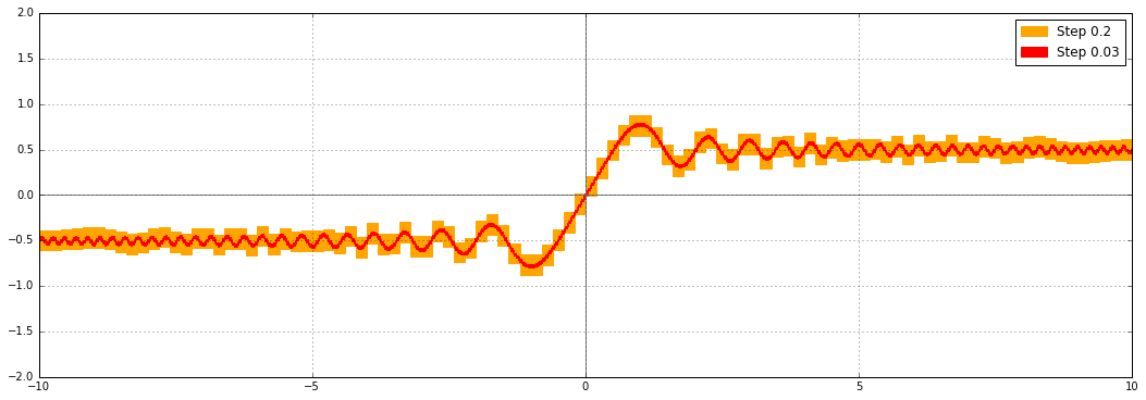
The proper solution is to evaluate $\operatorname{erf}([x \pm \delta])$ by evaluating $\operatorname{erf}(x)$ at the exact midpoint with increased precision, and separately bounding the error due to omitting $\delta$ (see: generic first-order bound). For the error function, error propagation can use the simple explicit formula $\operatorname{erf}\,'(x) = 2 e^{-x^2} / \sqrt{\pi}$. In recent commits (mainly this), I implemented this improvement for erf and erfc. This is what erf looks like now:
For the complementary error function, automatically increasing the precision helps for precise input as well. Previously, at 53-bit precision and with 15-digit printing, you would get:
erfc(1) = [0.15729920705029 +/- 6.87e-15]
erfc(2) = [0.00467773498105 +/- 5.88e-15]
erfc(3) = [2.20904970e-5 +/- 1.28e-14]
erfc(4) = [1.54173e-8 +/- 4.64e-14]
erfc(5) = [1.5e-12 +/- 6.17e-14]
erfc(6) = [+/- 3.56e-14]
erfc(7) = [4.1838256077794e-23 +/- 2.29e-37]      # asymptotic expansion used from here
erfc(8) = [1.12242971729829e-29 +/- 4.09e-44]
erfc(9) = [4.1370317465138e-37 +/- 1.54e-51]
Now, you get:
erfc(1) = [0.157299207050285 +/- 1.53e-16]
erfc(2) = [0.00467773498104727 +/- 4.49e-18]
erfc(3) = [2.20904969985854e-5 +/- 4.81e-20]
erfc(4) = [1.54172579002800e-8 +/- 2.17e-23]
erfc(5) = [1.53745979442803e-12 +/- 5.16e-27]
erfc(6) = [2.15197367124989e-17 +/- 1.98e-32]
erfc(7) = [4.1838256077794e-23 +/- 2.29e-37]
erfc(8) = [1.12242971729829e-29 +/- 3.56e-44]
erfc(9) = [4.13703174651381e-37 +/- 9.27e-52]
An alternative way to produce tight output intervals for erf and erfc would be to evaluate the function at both endpoints of the interval. However, this only works for monotone functions, and it requires two function evaluations instead of one. The midpoint+radius method also works for oscillatory functions and functions of complex variables. In fact, the worst case for computing erf or erfc is along the diagonals $z = (1 \pm i) x$ in the complex plane, where the asymptotic expansion transitions between exponential growth on one side of the diagonal and exponential decay on the other (the behavior on the diagonal itself is oscillatory). Up to normalizing factors, the error function on the diagonals is equivalent to the Fresnel integrals. Specifically, $$\tfrac{1}{2} (1+i) \operatorname{erf}(\tfrac{1}{2} \sqrt{\pi} (1 \pm i) z) = C(z) \pm i S(z)$$ where $S(z) = \int_0^z \sin(\tfrac{1}{2} \pi t^2) dt$ and $C(z) = \int_0^z \cos(\tfrac{1}{2} \pi t^2) dt$.
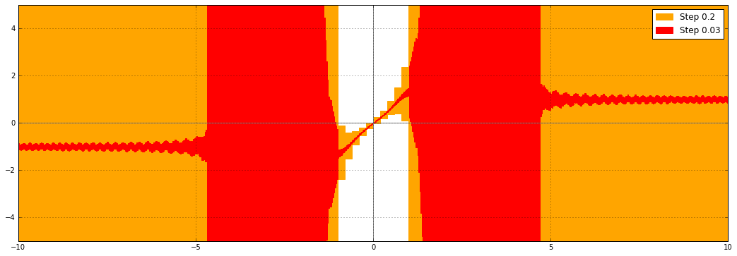
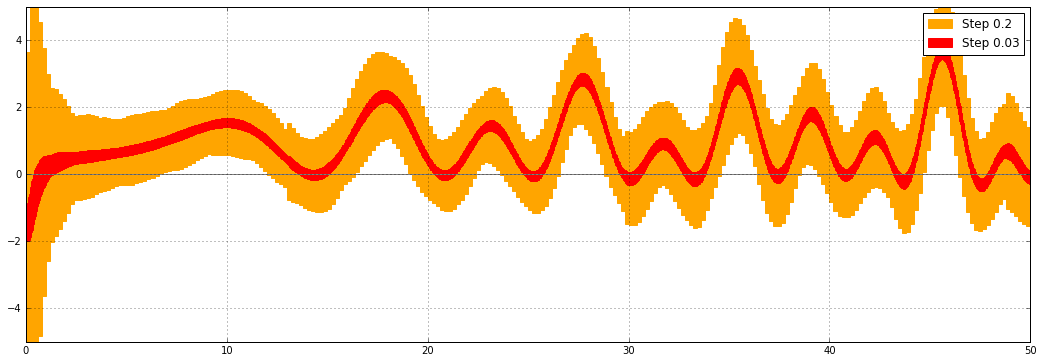
Here is a plot of the real part of $\operatorname{erf}((1+i)x)$ with the old version of the code:
Here it is with the new code:
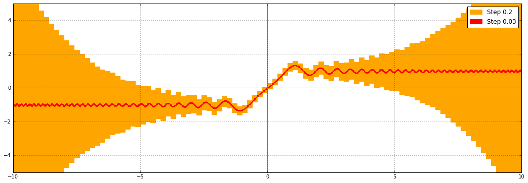
There is a vast improvement, but something funny is still happening as $|x| \to \infty$. Although the function is bounded on the diagonal $z = (1+i) x$, $x \in \mathbb{R}$, the bounds are still growing, slowly. Why? The problem is actually not with the implementation of the error function, but with the complex interval format. We want to evaluate the function on a diagonal line segment $(1+i) \cdot [a,b]$ in the complex plane, but complex numbers in Arb are represented by rectilinear boxes, so the actual input will be $[a,b] + [a,b] i$:
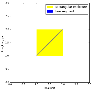
This inability to track the precise geometrical shape of the input is known as the wrapping effect. As a consequence, the complex interval passed to erf includes points not lying on the diagonal. Slightly off the the diagonal, erf diverges from the values right on the diagonal, and the computed error bounds correctly account for this fact.
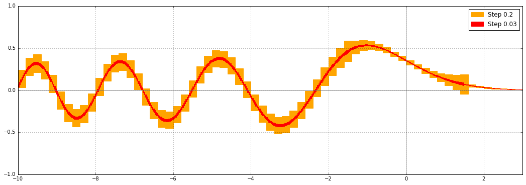
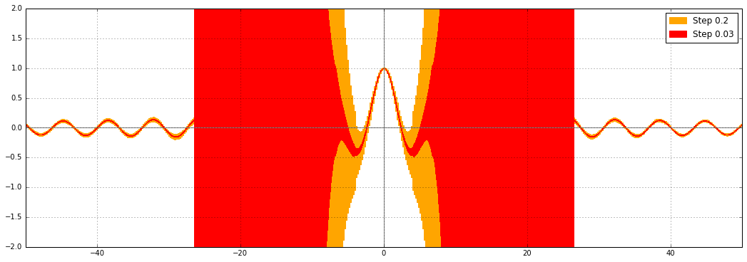
The solution is to implement Fresnel integrals as separate functions. Instead of diagonal line segments in the complex plane, the inputs can be real line segments (as long as we are interested in the Fresnel integrals on the real line), so the wrapping effect vanishes. I implemented the Fresnel integrals in Arb, and this is what $C(x)$ looks like on the real line:
That looks very nice indeed. Here is the Python code I used to produce the error plots. It depends on the experimental python-flint wrapper to call Arb functions.
%matplotlib inline
import flint
import mpmath
import matplotlib.pyplot as plt
import matplotlib.patches as patches
import pylab
import matplotlib.patches as mpatches
from numpy import arange
from flint import arb, acb

plt.clf()
ax = plt.gca()
legends = []

def ploterr(ax, f, xab, yab, step, yrange=None, color=None):
    xrad = step * 0.5
    a, b = xab
    top = 0.0
    bot = 0.0
    ax.axhline(color="gray")
    ax.axvline(color="gray")
    for xx in arange(a,b,2*xrad):
        xmid = xx + xrad
        X = arb(xmid, xrad)
        Y = f(X)
        if Y.is_finite():
            ymid = float(arb(Y.mid()))
            yrad = float(arb(Y.rad()))
            top = max(top, (ymid + yrad) * 1.2)
            bot = min(bot, (ymid - yrad) * 1.2)
            ax.add_patch(patches.Rectangle((xmid-xrad, ymid-yrad), 2*xrad, 2*yrad, color=color))
        else:
            ax.add_patch(patches.Rectangle((xmid-xrad, -1e50), 2*xrad, 1e50, color=color))
    ax.set_xlim([a,b])
    if yab is None:
        ax.set_ylim([bot,top])
    else:
        ax.set_ylim(yab)
    ax.grid(True)
    patch1 = mpatches.Patch(color=color, label='Step %s' % step)
    legends.append(patch1)

#ploterr(ax, lambda X: acb(X).erf().real, [-6, 6], [-2,2], 0.2, color="orange")
#ploterr(ax, lambda X: acb(X).erf().real, [-6, 6], [-2,2], 0.03, color="red")

#ploterr(ax, lambda X: acb(X,X).erf().real, [-10, 10], [-5,5], 0.2, color="orange")
#ploterr(ax, lambda X: acb(X,X).erf().real, [-10, 10], [-5,5], 0.03, color="red")

ploterr(ax, lambda X: acb(X).fresnel_c().real, [-10, 10], [-2,2], 0.2, color="orange")
ploterr(ax, lambda X: acb(X).fresnel_c().real, [-10, 10], [-2,2], 0.03, color="red")

ax.legend(handles=legends)
import matplotlib
fig = matplotlib.pyplot.gcf()
fig.set_size_inches(18, 6)
fig.savefig('test.png')
It's fun to try it with different builtin Arb functions: some are computed with very good error bounds, others not so much. There are many other functions that need to get the same treatment as erf, but doing so is often hard, because most mathematical functions don't have a convenient way to bound the derivative tightly.
The Airy functions are examples with good error bounds:
The Riemann zeta function on the critical line (here the real part) has decent, but not great, error bounds:
The gamma function leaves something to be desired (this has been on my todo list for a while):
Bessel functions (here $J_0(x)$) still suffer from the problem that erf had; also on my todo list:
fredrikj.net |
Blog index |
 RSS feed |
Follow me on Mastodon |
Become a sponsor
RSS feed |
Follow me on Mastodon |
Become a sponsor