fredrikj.net / blog /
The Arb matrix reloaded
June 29, 2018
Basic linear algebra in Arb is getting a significant upgrade in Arb 2.14 which is due to be released within a few weeks. The main improvements are more accurate linear solving and faster matrix multiplication.
Linear solving
The current development version of Arb (2.14-git) offers a dramatic improvement for solving large well-conditioned linear systems. To illustrate this, the following program constructs and solves $AX = B$ where $A$ is an $n \times n$ real matrix and $B$ is an $n \times 1$ vector. The program starts with 53-bit precision and doubles the precision until arb_mat_solve succeeds to prove that the matrix is invertible. The program then terminates and prints the first, middle and last entry in the solution vector with up to 20 digits. We take $n = 1000$ and we set $A$ to the size-$n$ discrete cosine transform (DCT) matrix with entries $$A_{j,k} = \sqrt{\frac{2}{n}} \cos\left(\tfrac{\pi j}{n} \left(k+\tfrac{1}{2}\right)\right).$$ We set $B$ to the vector of all ones. No special properties of the DCT matrix are being used here; it is just a convenient test matrix that is well-conditioned (the function arb_mat_dct used to create this matrix is a new addition to Arb; some other functions to generate useful special matrices have also been added).
#include "arb_mat.h"
#include "flint/profiler.h"

int main()
{
    arb_mat_t A, B, X;
    slong prec, n;
    n = 1000;
    arb_mat_init(A, n, n);
    arb_mat_init(B, n, 1);
    arb_mat_init(X, n, 1);
    TIMEIT_START
    for (prec = 53; ; prec *= 2)
    {
        printf("prec = %ld\n", prec);
        arb_mat_dct(A, 0, prec);
        arb_mat_ones(B);
        if (arb_mat_solve(X, A, B, prec))
        {
            arb_printn(X->rows[0], 20, 0); printf("\n");
            arb_printn(X->rows[X->r/2], 20, 0); printf("\n");
            arb_printn(X->rows[X->r-1], 20, 0); printf("\n");
            break;
        }
    }
    TIMEIT_STOP
    arb_mat_clear(A);
    arb_mat_clear(B);
    arb_mat_clear(X);
    return 0;
}
This is the before and after comparison:
| Arb 2.13 | Arb 2.14-git |
|---|---|
prec = 53 prec = 106 prec = 212 prec = 424 prec = 848 prec = 1696 [+/- 2.99e+14] [0.031587680085551469491 +/- 4.08e-22] [0.0092445347862472445663 +/- 2.78e-24] cpu/wall(s): 442.749 442.805 |
prec = 53 [28.47975797950 +/- 7.97e-12] [0.031587680086 +/- 5.06e-13] [0.0092445347862 +/- 9.55e-14] cpu/wall(s): 18.348 18.349 |
The old version of arb_mat_solve uses direct Gaussian elimination to compute the LU factorization of the system matrix. This is numerically unstable in interval arithmetic in general, even when the system is well-conditioned. The precision needed for convergence scales like $O(n)$ and in this case exceeds 1000 bits. In fact, even after the solving succeeds, the top entry in the solution vector is wildly imprecise and we would have to double the precision one more time to get it precise.
The new version of arb_mat_solve completes 24 times faster, and more importantly, succeeds directly at 53-bit precision with only a few digits of precision loss! As a reference point, we can evaluate the matrix-vector product $A^T B$ (which is mathematically equivalent to $A^{-1} B$ for this $A$ since the DCT matrix is orthogonal); the corresponding entries then come out as:
[28.47975797950 +/- 2.78e-12]
[0.0315876800856 +/- 6.38e-14]
[0.0092445347862 +/- 6.03e-14]
We see that the error bounds from arb_mat_solve are just a small factor larger than the optimal bounds. This is a big deal in applications where the input matrices may be expensive to generate at high precision. In fact, arb_mat_solve still succeeds on the first try if we set the starting precision to 20 bits (and this is even faster):
prec = 20
[2.8e+1 +/- 0.505]
[0.032 +/- 9.06e-4]
[0.009 +/- 6.61e-4]
cpu/wall(s): 12.385 12.396
The main ingredient in the new arb_mat_solve is the Hansen-Smith algorithm from 1967. Instead of solving $AX = B$ directly, we compute an approximate inverse matrix $R \approx A^{-1}$ and then solve the preconditioned system $(RA)X = RB$. Gaussian elimination on the matrix $RA \approx I$ is numerically stable even in interval arithmetic (in fact, in some cases we can just bound the perturbation away from the identity matrix and skip the last solving step entirely). Computing $R$ can be done heuristically with the usual floating-point Gaussian elimination, and ball arithmetic only enters when computing $RA$, $RB$ and in the last solving step. The credit for implementing this algorithm in Arb goes to a contributor who wished to remain anonymous.
The drawback, of course, is that we are doing 3-4 times more work than just running Gaussian elimination once. This slowdown is offset to some extent by another improvement: I have rewritten Gaussian elimination to use a block recursive strategy which takes advantage of matrix multiplication, and matrix multiplication has been optimized (see below).
The following plot and table compare the performance on the DCT matrix benchmark as the dimension $n$ varies:
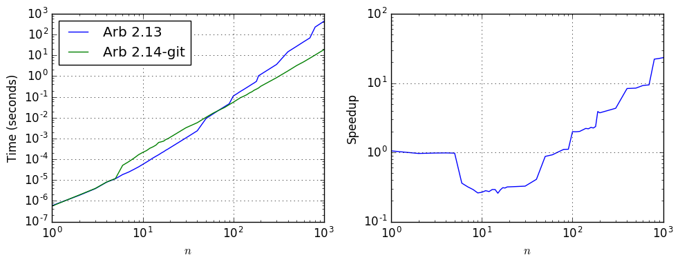
| $n$ | Time, Arb 2.13 | Time, Arb 2.14-git | Speedup |
|---|---|---|---|
| 10 | 5.68e-05 | 0.000214 | 0.26 |
| 30 | 0.00107 | 0.00329 | 0.33 |
| 100 | 0.111 | 0.0558 | 1.99 |
| 300 | 3.658 | 0.845 | 4.33 |
| 1000 | 442.749 | 18.348 | 24.1 |
For sizes from about to 6 to 50 where the old algorithm succeeds without increasing the precision (for this particular matrix), the new algorithm is about three times slower, but the improvement in accuracy is dramatic. Here showing the first entry in the output vector, for different $n$:
n     Arb 2.13                          Arb 2.14-git
======================================================================
5     [2.1275693661542 +/- 5.10e-14]    [2.1275693661542 +/- 5.10e-14]
6     [2.3122784967091 +/- 8.64e-14]    [2.3122784967091 +/- 2.12e-14]
7     [2.482712359015 +/- 3.50e-13]     [2.4827123590148 +/- 5.33e-14]
8     [2.641845987495 +/- 7.03e-13]     [2.6418459874955 +/- 2.08e-14]
9     [2.79172023714 +/- 3.30e-12]      [2.7917202371376 +/- 4.33e-14]
10    [2.93381472088 +/- 9.40e-12]      [2.9338147208785 +/- 1.04e-14]
15    [3.55934770 +/- 1.52e-9]          [3.5593476994815 +/- 3.07e-14]
20    [4.089760 +/- 5.21e-7]            [4.0897599643974 +/- 6.84e-14]
25    [4.559 +/- 4.29e-4]               [4.5586791661163 +/- 6.77e-14]
30    [5.0 +/- 0.0546]                  [4.9835836367848 +/- 5.87e-14]
35    [+/- 11.3]                        [5.3749570875008 +/- 5.67e-14]
40    [+/- 6.55e+3]                     [5.7396790611281 +/- 6.55e-14]
45    [+/- 3.93e+5]                     [6.082554137056 +/- 2.18e-13]
Using the slower but more accurate algorithm by default seems like a sensible tradeoff since losing several significant digits may be much more costly overall when propagated through a larger computation. It should be noted that the code switches back to direct Gaussian elimination when the precision is much higher than the expected precision loss, so no slowdown will occur when solving 20 by 20 systems at 1000-digit precision, for example. Users also have the option of selecting an algorithm manually by calling arb_mat_solve_lu (direct Gaussian elimination) or arb_mat_solve_precond (the Hansen-Smith algorithm) instead of the default arb_mat_solve.
Versus the machine
With $n = 1000$ and 53-bit precision, the new arb_mat_solve is "only" 150 times slower than numpy.linalg.solve (LAPACK dgesv) which takes 0.125 seconds to compute a non-certified solution. Roughly one order of magnitude is due to the inherent overhead of the certified solving algorithm, and another order of magnitude is due to using arbitrary-precision arithmetic. The second item is certainly improvable: a factor two could be saved by using double internally for the approximate solving, and another factor three could probably be saved with use of BLAS and other optimizations in FLINT. This would bring the factor down to 25 which is in the ballpark of machine-precision interval software such as INTLAB which reportedly solves a size-1000 system 12 times slower than MATLAB's backslash operator. In principle, the solving in Arb at precision up to 53 bits could be made nearly as fast as INTLAB by converting the matrices to double format and doing all calculations (including certifications) in this format internally. Implementing this correctly is complicated, however, and the design is more conservatively structured around arbitrary-precision arithmetic for now.
Ill-conditioned systems
For solving ill-conditioned systems, increasing the precision (typically to $O(n)$ bits) is unavoidable. If we change the DCT matrix to a Hilbert matrix, the old and new versions of arb_mat_solve compare as follows:
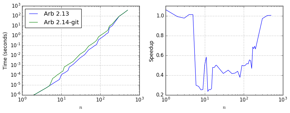
| $n$ | Time, Arb 2.13 | Time, Arb 2.14-git | Speedup |
|---|---|---|---|
| 10 | 0.00010 | 0.000203 | 0.49 |
| 30 | 0.00529 | 0.0128 | 0.41 |
| 100 | 0.5 | 1.013 | 0.49 |
| 300 | 85.362 | 87.791 | 0.97 |
Again, a slight slowdown for ill-conditioned systems is a necessary tradeoff to optimize for well-conditioned systems and for global efficiency, and users who know that they are dealing with a system of this type in the range where direct Gaussian elimination is faster can always call arb_mat_solve_lu manually.
Matrix inversion
The improved linear solving also extends to matrix inversion, which just amounts to solving $AX = I$. In fact, the new code performs even better in this case compared to the old code: with the old code, solving with a square matrix right-hand side is about twice as expensive as with a vector right-hand side, but with the new algorithm, a matrix right-hand side is barely more expensive than a vector.
If we change the DCT benchmark code above to compute $A^{-1}$ (by calling arb_mat_inv instead of arb_mat_solve), we find that Arb 2.14-git is 50 times faster than Arb 2.13 when $n = 1000$.
Matrix multiplication
Matrix multiplication in Arb previously just used the classical algorithm, executed in ball arithmetic (arb_mat_mul_classical). There is also a multithreaded version (arb_mat_mul_threaded) of classical multiplication that helps for large matrices if the user has a lot of cores available. However, the classical algorithm is not ideal for arbitary-precision arithmetic, because there is a huge amount of overhead for each arithmetic operation.
Polynomial multiplication in Arb uses the trick of breaking the polynomials into blocks of coefficients that have nearly the same magnitude, rescaling these blocks to have integer coefficients, and multiplying the individual blocks using FLINT's blazingly fast $\mathbb{Z}[x]$ (fmpz_poly) arithmetic. The new matrix multiplication code in Arb 2.14-git uses an analogous scheme for matrices, multiplying blocks of coefficients with similar magnitude via FLINT's fmpz_mat.
The algorithm in more detail
The code implements a scaling trick for individual blocks: if $A_i$ and $B_i$ are the submatrices to be multiplied, the algorithm inspects the exponent changes along rows of $A_i$ and along columns of $B_i$ to determine diagonal matrices (specifically, with power-of-two entries) $D_1$ and $D_2$ such that $D_1 A_i$ and $B_i D_2$ are integer matrices with nearly minimal height. It then evaluates $A_i B_i = D_1^{-1} (D_1 A_i) (B_i D_2) D_2^{-1}$.
If the input matrices $A$ and $B$ have coefficients of nearly uniform magnitude (in individual rows of $A$ and columns of $B$), a single block $A = A_i$ and $B = B_i$ can be used. The complicated part of the algorithm is to split non-uniformly scaled matrices into blocks that are optimal for efficiency. On one hand, the blocks should be as large as possible, since this makes fmpz_mat matrix multiplication more advantageous. On the other hand, when the coefficient magnitudes vary, larger blocks result in larger integers which slows things down. I have implemented a fairly simple heuristic which consists of greedily scanning forward for maximal consecutive spans of columns of $A$ and rows of $B$ that fit within a limited exponent range. I make no claims that this is the best way to do it, but it works reasonably well.
Integer matrix multiplication is a bit faster already for small matrices since it has less overhead than ball arithmetic. It becomes much faster for huge matrices (say $n > 100$) since it can use a multimodular algorithm performing one or several matrix multiplications modulo single-word primes. FLINT also uses Strassen multiplication so the complexity is in fact $O(n^{2.81})$ and not $O(n^3)$.
Integer matrices are used for the multiplying the matrices of midpoints. When the matrices are inexact, say $A = A_m \pm A_r$ and $B = B_m \pm B_r$, the two additional matrix products $(|A_m| + A_r) B_r$ and $A_r |B_m|$ are computed by splitting into scaled blocks and using double arithmetic. This is faster and works well since all entries are nonnegative making it trivial to compute tight upper bounds.
One could implement Strassen multiplication and other tricks directly in Arb, but this is not a good idea in most cases since it is less numerically stable than classical matrix multiplication. The new matrix multiplication code is designed to give at least as good error bounds as the classical algorithm for every individual coefficient in the output. In fact, the error bounds are usually a bit better since fewer internal rounding operations are performed.
Future improvements are certainly possible. Matrix multiplication in FLINT could probably be sped up by about a factor three using BLAS and other optimizations (FLINT currently uses non-vectorized 64-bit integer arithmetic for modular matrix multiplications and has unoptimized basecase code for modular reduction and Chinese remaindering).
Some benchmarks
I have done a bit of benchmarking with three families of test matrices:
- Hilbert matrices, with entries $A_{i,j} = 1/(i+j+1)$. These are (for the purposes of multiplication) generic real matrices with uniformly scaled entries, which can be multiplied using a single block.
- Small-integer matrices, with entries $A_{i,j} = i + j + 1$.
- Pascal matrices (times a constant factor), with entries $A_{i,j} = \pi \cdot {i+j \choose i}$. Since binomial coefficients grow rapidly (${2 n \choose n} \approx 4^n$), these matrices are a bad case for the multiplication algorithm, requiring splitting into many smaller blocks when $n$ is large. The factor $\pi$ makes the entries generic full-precision real numbers instead of integers.
For this test, we set both operands to the same matrix, and we compare multiplication speed at a precision of 53, 128, 333 and 1024 bits.
Hilbert matrices
The following plot shows the timings for Hilbert matrices. The different levels of precision are indicated with different colors and in the left subplot, the timings for the old code are shown as dashed curves while the timings for the new code are shown as solid curves:
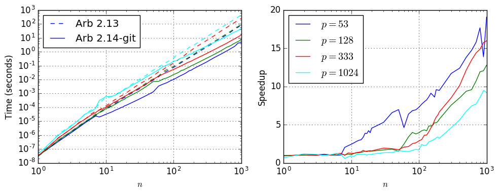
At 1-2 words of precision, the new code is five times faster than the old code even for relatively small matrices and a factor 20 faster for matrices with dimension $n$ in the thousands. The time for an $n = 1000$ matrix multiplication is down from two minutes to 4-10 seconds. At hundreds of digits, the advantage of the new algorithm is starting to diminish but there is still a large speedup as soon as the dimension also gets large.
| $p$ | $n$ | Time, Arb 2.13 | Time, Arb 2.14-git | Speedup |
|---|---|---|---|---|
| 53 | 10 | 7.8e-05 | 3.2e-05 | 2.44 |
| 53 | 30 | 0.00191 | 0.00036 | 5.31 |
| 53 | 100 | 0.075 | 0.0103 | 7.28 |
| 53 | 300 | 2.014 | 0.172 | 11.7 |
| 53 | 1000 | 89.329 | 4.681 | 19.1 |
| $p$ | $n$ | Time, Arb 2.13 | Time, Arb 2.14-git | Speedup |
|---|---|---|---|---|
| 128 | 10 | 8.9e-05 | 8.3e-05 | 1.07 |
| 128 | 30 | 0.00229 | 0.00135 | 1.70 |
| 128 | 100 | 0.091 | 0.0231 | 3.94 |
| 128 | 300 | 2.428 | 0.321 | 7.56 |
| 128 | 1000 | 95.169 | 7.443 | 12.8 |
| $p$ | $n$ | Time, Arb 2.13 | Time, Arb 2.14-git | Speedup |
|---|---|---|---|---|
| 333 | 10 | 0.000129 | 0.000103 | 1.25 |
| 333 | 30 | 0.0043 | 0.00222 | 1.94 |
| 333 | 100 | 0.155 | 0.054 | 2.87 |
| 333 | 300 | 6.038 | 0.708 | 8.53 |
| 333 | 1000 | 257.607 | 16.122 | 16.0 |
| $p$ | $n$ | Time, Arb 2.13 | Time, Arb 2.14-git | Speedup |
|---|---|---|---|---|
| 1024 | 10 | 0.00056 | 0.00062 | 0.90 |
| 1024 | 30 | 0.0093 | 0.007 | 1.33 |
| 1024 | 100 | 0.371 | 0.218 | 1.70 |
| 1024 | 300 | 11.111 | 2.41 | 4.61 |
| 1024 | 1000 | 454.495 | 49.298 | 9.22 |
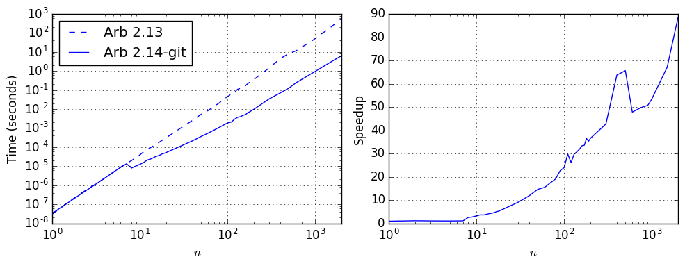
Small-integer matrices
The speedup is even more dramatic when multiplying Arb matrices with small integer entries. This is now essentially as fast as using fmpz_mat directly, up to the conversion overhead. The plot below compares the performance for multiplying the matrices with entries $A_{i,j} = B_{i,j} = i + j + 1$. A single $n = 1000$ multiplication now takes one second, down from a minute, and the speedup continues to grow to a factor 100 beyond $n = 2000$.
| $p$ | $n$ | Time, Arb 2.13 | Time, Arb 2.14-git | Speedup |
|---|---|---|---|---|
| 53 | 10 | 4e-05 | 1.26e-05 | 3.17 |
| 53 | 30 | 0.0011 | 0.000121 | 9.09 |
| 53 | 100 | 0.045 | 0.00188 | 23.9 |
| 53 | 300 | 1.495 | 0.035 | 42.7 |
| 53 | 1000 | 50.957 | 0.955 | 53.4 |
| 53 | 2000 | 568.174 | 6.412 | 88.6 |
(Here, the precision does not matter; the matrices and their product are exactly representable at 53-bit precision, and increasing the precision does not cause any slowdown.)
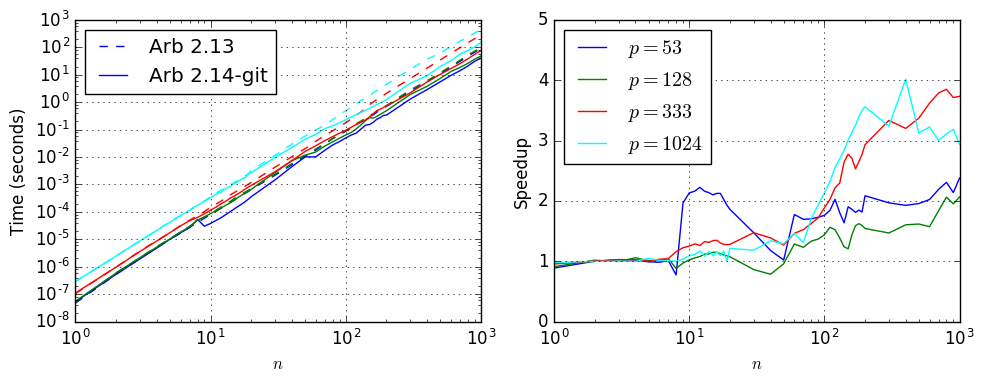
Pascal matrices
With Pascal matrices (multiplied by the factor $\pi$), the speedup is modest due to the need to use many blocks. Nevertheless, for large enough $n$, the new algorithm saves a factor 2-4 depending on the precision.
| $p$ | $n$ | Time, Arb 2.13 | Time, Arb 2.14-git | Speedup |
|---|---|---|---|---|
| 53 | 10 | 8.1e-05 | 3.8e-05 | 2.13 |
| 53 | 30 | 0.00218 | 0.00148 | 1.47 |
| 53 | 100 | 0.088 | 0.05 | 1.76 |
| 53 | 300 | 2.569 | 1.305 | 1.97 |
| 53 | 1000 | 96.37 | 40.518 | 2.38 |
| $p$ | $n$ | Time, Arb 2.13 | Time, Arb 2.14-git | Speedup |
|---|---|---|---|---|
| 128 | 10 | 8.9e-05 | 8.7e-05 | 1.02 |
| 128 | 30 | 0.00237 | 0.00275 | 0.86 |
| 128 | 100 | 0.092 | 0.064 | 1.44 |
| 128 | 300 | 2.819 | 1.92 | 1.47 |
| 128 | 1000 | 100.019 | 48.427 | 2.07 |
| $p$ | $n$ | Time, Arb 2.13 | Time, Arb 2.14-git | Speedup |
|---|---|---|---|---|
| 333 | 10 | 0.000145 | 0.000116 | 1.25 |
| 333 | 30 | 0.0043 | 0.00292 | 1.47 |
| 333 | 100 | 0.179 | 0.095 | 1.88 |
| 333 | 300 | 7.371 | 2.21 | 3.34 |
| 333 | 1000 | 288.91 | 77.335 | 3.73 |
| $p$ | $n$ | Time, Arb 2.13 | Time, Arb 2.14-git | Speedup |
|---|---|---|---|---|
| 1024 | 10 | 0.00036 | 0.00033 | 1.09 |
| 1024 | 30 | 0.0116 | 0.0098 | 1.18 |
| 1024 | 100 | 0.493 | 0.231 | 2.13 |
| 1024 | 300 | 16.088 | 4.965 | 3.24 |
| 1024 | 1000 | 453.439 | 154.31 | 2.94 |
Complex matrices and more
Implementing fast multiplication, solving and matrix inverse for complex matrices (acb_mat) is a work in progress that will be finished before Arb 2.14 is released.
Determinants of real and complex matrices can also be improved using similar preconditioning tricks, but this requires a separate implementation which might be postponed until later.
fredrikj.net |
Blog index |
 RSS feed |
Follow me on Mastodon |
Become a sponsor
RSS feed |
Follow me on Mastodon |
Become a sponsor