fredrikj.net / blog /
Computing the Lerch transcendent
February 18, 2022
The Lerch transcendent is a useful special function of three complex variables, initially defined by the series $$\Phi(z,s,a) = \sum_{n=0}^{\infty} \frac{z^n}{(n+a)^s}, \quad |z| < 1$$ and extended by analytic continuation to the complex $z$-plane with the exception of a singularity at $z = 1$ and a branch cut on $z \in [1, +\infty)$. The Lerch transcendent can be viewed as a generalization of several important special functions: special cases include the usual geometric series ($s = 0$), the natural logarithm ($a = 1, s = 1$), powers and exponentials ($z = 0$), polylogarithms ($a = 1$), the Riemann zeta function ($z = a = 1$), the alternating Riemann zeta function ($z = -1, a = 1$), and the Hurwitz zeta function ($z = 1$).
The Lerch transcendent has sadly been missing from Arb, but I finally added a first implementation a couple of days ago. Below, I will discuss the strategy to compute the function rigorously for arbitrary complex parameters. I will also briefly discuss some algorithms that are not currently implemented. The Arb code is not very optimized (especially for large parameters), but it does the job and can serve as a baseline for trying out more efficient algorithms in the future.
Contents
A look at Lerch
Before diving into the details, here are two complex-domain plots generated with Arb.
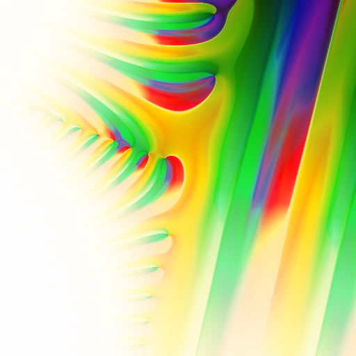
As a function of $z$, the Lerch transcendent behaves like a deformed logarithm:

Domain coloring plot of $\Phi(z, 1+3i, 2-i)$ on $s \in [-5,5] + [-5,5] i$.
As a function of $s$, the Lerch transcendent behaves like a deformed Riemann zeta function:
Domain coloring plot of $\Phi(-0.75 i, s, 1-0.5 i)$ on $s \in [-20,20] + [-20,20] i$.
Direct series
The defining series can be used directly when $|z| \le 0.9$, say (near $|z| \approx 1$ convergence becomes very slow). The truncation error after adding $N$ terms can be bounded by a geometric series as follows. We have, for large enough $N$, $$\left|\sum_{n=N}^{\infty} \frac{z^n}{(n+a)^s}\right| = \left|z^N (N+a)^{-s} \sum_{n=0}^{\infty} z^n (1 + (N+a)^{-1} n)^{-s}\right| \le |z^N (N+a)^{-s}| \sum_{n=0}^{\infty} (C |z|)^n = \frac{|z^N (N+a)^{-s}|}{1 - C |z|}$$ for some constant $C$ satisfying $C |z| < 1$. Choose $N$ so that $\operatorname{Re}(N + a) > 0$ and define $\alpha = (N + a)^{-1}$. If $a$ is real, we may use the inequality $$|(1 + \alpha n)^{-s}| \le C^n, \quad C = \exp(\max(0, -\operatorname{Re}(s)) \alpha).$$ Otherwise, we may use $$|(1 + \alpha n)^{-s}| \le C^n, \quad C = \exp(|s \alpha|).$$ This last bound can be quite pessimistic when the parameters get large, but it works well enough for moderate parameters (as already mentioned, I have not attempted to optimize for large parameters).
Choosing $N$ for a given level of precision is easy: just evaluate the error bound for a sequence of increasing $N$ until the bound is smaller than the target error.
To evaluate the truncated series in high-precision arithmetic, there is not much to improve over the naive algorithm unless $s$ is a small integer in which case hypergeometric/holonomic methods could be used (not implemented). For generic (noninteger) $s$, the bulk of the work is to evaluate $(n+a)^{-s} = \exp(-s \log(n+a))$, requiring two transcendental function calls per term. Gradually decreasing the working precision along with the magnitude of the terms would help a bit at high precision.
Laplace transform integral
The main tool to compute the analytic continuation of $\Phi(z,s,a)$ will be numerical integration. We have the following Laplace transform-type integral representation: $$\Phi(z,s,a) = \frac{1}{\Gamma(s)} \int_0^{\infty} \frac{t^{s-1} e^{-a t}}{1 - z e^{-t}} dt.$$
We can use the adaptive complex Gaussian integration in Arb to evaluate this type of integral efficiently (see a previous blog post about computing special functions using integration and an older post about the integration algorithm itself).
Truncation
Since Gaussian integration works on finite intervals, we need to truncate the integral at some upper limit $R$. We can bound the truncation error as follows. Define $\sigma = \operatorname{Re}(s)$, $\alpha = \operatorname{Re}(a)$. If $R > |\log(z)| + 1$, then $$\left| \int_R^{\infty} \frac{t^{s-1} e^{-a t}}{1 - z e^{-t}} dt \right| \le 2 C^{-1} R^{\sigma-1} e^{-\alpha R}, \quad C = \alpha - \frac{\max(0, \sigma - 1)}{R}$$ if $C > 0$. (To prove this, we note that the contribution of the denominator of the integrand is bounded by a factor $|1 - z e^{-R}|^{-1} \le |1 - z |z|^{-1} e^{-1}|^{-1} < 2$. Next, $$\left| \int_R^{\infty} t^{s-1} e^{-at} dt \right| = \left| R^{s-1} e^{-a R} \int_0^{\infty} e^{-a t} \left(1 + \frac{t}{R}\right)^{s-1} dt \right|$$ and the integrand on the right is bounded by $\exp(-\alpha t + \max(0, \sigma-1) t / R)$. Inserting this bound, the integral can be done in closed form.) The easiest way to choose an appropriate value $R$ here is to simply try several successive values and stop when the bound is small enough.
Restrictions and workarounds
The integral representation stated above is only valid subject to the following restrictions:
- $z \not \in [1,\infty)$
- $\operatorname{Re}(s) > 0$
- $\operatorname{Re}(a) > 0$
We will now discuss how to lift all these restrictions. The restriction $\operatorname{Re}(a) > 0$ is very easily circumvented because we can shift this parameter arbitrarily far to the right using the recurrence relation $$\Phi(z,s,a) = z^n \Phi(z,s,a+n) + \sum_{k=0}^{n-1} \frac{z^k}{(k+a)^s}.$$
To deal with $z$ near the branch cut of $\Phi(z,s,a)$ (i.e. $\log(z)$ near the real line), we can deform the path of integration as follows:

The Arb implementation uses the original straight-line path on $[0,+\infty)$ when $\operatorname{Re}(\log(z)) < 0$ or $|\operatorname{Im}(\log(z))| > 0.25$, and otherwise deforms the contour to stay clear of the poles. We take the detour through the lower half plane (as pictured) if $\operatorname{Im}(\log(z)) > 0$ and through the upper half plane (the mirror image of the diagram) if $\operatorname{Im}(\log(z)) \le 0$. This ensures counterclockwise continuity of the principal branch of $\Phi(z,s,a)$ on the cut, consistent with the usual convention for the logarithm. The path of integration must not be deformed so far that it goes around any other poles; fortunately, the poles are always well separated (by a distance $2 \pi$), so this is not an issue.
Avoiding the restriction on $s$ is a bit more involved. In fact, numerically speaking there is a problem for noninteger $s$ even when the integral converges, because the algebraic singularity slows down the integration algorithm. The Arb implementation therefore only uses the above form of the integral for $s \in \{1, 2, \ldots\}$.
Hankel contour
To construct an algorithm that works for general $s$, we will use the following version of the integral (see Erdélyi et al., section 1.11.): $$\Phi(z,s,a) = -\frac{\Gamma(1-s)}{2 \pi i} \int_H \frac{(-t)^{s-1} e^{-a t}}{1 - z e^{-t}} dt.$$ This integral is valid for $z \not \in [1, \infty)$, $s \not \in \{1, 2, \ldots\}$ and $\operatorname{Re}(a) > 0$ (the last restriction can be removed using recurrence relations as described above). Here, $H$ is a Hankel contour starting at $+\infty$ in the upper half plane, circling around the origin and returning to $+\infty$ in the lower half plane, without enclosing any poles of the integrand. This avoids the singularity at $t = 0$ entirely:

Note that by changing the power in the integrand from $t^{s-1}$ to $(-t)^{s-1}$, we have moved the branch cut of the integrand from the negative half line to the positive half line, and the Hankel contour does not cross this branch cut, so the integrand is holomorphic on the entire path. The gamma factor unfortunately means that the formula is not valid for $s \in \{1, 2, \ldots\}$, but in that case we can just use the original integral on the real line.
Now, a few crucial optimizations. We still have the issue that the method breaks down when $z$ is very close to (or on) the branch cut. The workaround is simple: if $\log(z)$ is too close to the positive real line (being located at a yellow dot instead of a red dot in the diagram below), we shift the contour away from the branch cut so that it definitely includes the pole, and then we subtract the residue.

In the right half-plane, we want to integrate $g(t) = t^{s-1} e^{-a t} (1 - z e^{-t})^{-1}$ rather than $h(t) = (-t)^{s-1} e^{-a t} (1 - z e^{-t})^{-1}$ so that the Gaussian integration can use large complex ellipses for the error bounds without the branch cut interfering. We have $g(t) = \omega h(t)$ in the upper half-plane and $g(t) = \omega^{-1} h(t)$ in the lower half-plane, where $\omega = (-1)^{s-1}$. After this rewriting, we can also deform the path again so that it becomes a closed loop plus a single ray towards infinity. The path can now be decomposed into the linear segments $I_1, \ldots, I_6$ illustrated above. Writing down the formulas, we have:
$$I = \omega^{-1} \left[\int_{I_1 \cup I_2} g(t) dt \right] + \int_{I_3} h(t) dt + \omega \left[\int_{I_4 \cup I_5} g(t) dt \right] + (\omega - \omega^{-1}) \int_{I_6} g(t) dt$$ $$\text{residue} = \begin{cases} \displaystyle \frac{(-\log(z))^s}{z^a \log(z)} & \text{if } \log(z) \text{ is inside the loop } \\ 0 & \text{otherwise} \end{cases}$$ $$\Phi(z,s,a) = -\Gamma(1-s) \left(\frac{I}{2 \pi i} + \text{residue}\right)$$Finally, there are some symmetries to exploit when all parameters are real. Wrapping it up, here is a basic Python implementation using mpmath:
def lerch_hankel(z, s, a):
    z, s, a = mpmathify(z), mpmathify(s), mpmathify(a)
    if z == 0 or z == 1 or mp.isnpint(a):
        return nan
    if re(a) < 2:
        return z * lerch_hankel(z, s, a + 1) + a**(-s)
    g = lambda t: t**(s-1)*exp(-a*t)/(1-z*exp(-t))
    h = lambda t: (-t)**(s-1)*exp(-a*t)/(1-z*exp(-t))
    L = log(z)
    if mp.isint(s) and re(s) >= 1:
        if abs(im(L)) < 0.25 and re(L) >= 0:
            if im(z) <= 0.0:
                I = quad(g, [0, +1j, +1j+abs(L)+1, abs(L)+1, inf])
            else:
                I = quad(g, [0, -1j, -1j+abs(L)+1, abs(L)+1, inf])
        else:
            I = quad(g, [0,inf])
        return rgamma(s) * I
    if re(L) < -0.5:
        residue = 0
        c = min(abs(re(L)) / 2, 1)
        left = right = top = c
    elif abs(im(L)) > 0.5:
        residue = 0
        c = min(abs(im(L)) / 2, 1)
        left = right = top = c
    else:
        residue = (-L)**s / L / z**a
        left = max(0, -re(L)) + 1
        top = abs(im(L)) + 1
        right = abs(L) + 1
    isreal = (im(z) == 0) and (re(z) < 1) and (im(s) == 0) and (im(a) == 0) and (re(a) > 0)
    w = mpc(-1)**(s-1)
    I = 0
    if isreal:
        I += 2j * im(quad(g, [right, right + top * 1j]) / w)
        I += 2j * im(quad(g, [right + top * 1j, -left + top * 1j]) / w)
        I += 2j * im(quad(h, [-left + top * 1j, -left]))
        I += quad(g, [right, inf]) * (w - 1/w)
    else:
        I += quad(g, [right, right + top * 1j]) / w
        I += quad(g, [right + top * 1j, -left + top * 1j]) / w
        I += quad(h, [-left + top * 1j, -left - top * 1j])
        I += quad(g, [-left - top * 1j, right - top * 1j]) * w
        I += quad(g, [right - top * 1j, right]) * w
        I += quad(g, [right, inf]) * (w - 1/w)
    I = I / (2*pi*1j) + residue
    I = -gamma(1-s) * I
    return I
The Arb implementation uses basically the same algorithm, except that there is some more work involved to truncate the integrals towards infinity (the heuristic numerical integration in mpmath is happy to do these directly), and some micromanagement is needed to avoid issues when the input balls for $z, s, a$ are wide and potentially overlapping different cases. I have not made any effort to optimize for large parameters using saddle-point analysis; there might also be some symmetries that I have overlooked.
Abel-Plana integral
There are other ways to construct the analytic continuation of the Lerch transcendent. An interesting method is the Abel-Plana formula which allows us to write an infinite series $\sum_{n=0}^{\infty} f(n)$ as a sum of two integrals (subject to some conditions on $f$): $$\sum_{n=0}^{\infty} f(n) = \frac{f(0)}{2} + \int_0^{\infty} f(t) dt + i \int_0^{\infty} \frac{f(it) - f(-it)}{e^{2 \pi t} - 1} dt.$$ There are also useful variations of this formula, for example $$\sum_{n=0}^{\infty} f(n) = f(0) + \int_{1/2}^{\infty} f(t) dt - i \int_0^{\infty} \frac{f(1/2+it) - f(1/2-it)}{e^{2 \pi t} + 1} dt$$ which avoids a removable singularity in the integrand at $t = 0$. For more precise statements of the Abel-Plana formula and applications, see section 4.2.4 in Belabas and Cohen.
If we apply the Abel-Plana formula to $f(n) = z^n / (n+a)^s$, we don't quite get an analytic continuation because the integral $\int_0^{\infty} f(t) dt$ only converges for $|z| < 1$ (or $|z| = 1$ with the right conditions on $s$). However, we may may note that this integral can be written in terms of another special function: the incomplete gamma function. We thus have
$$\Phi(z,s,a) = \frac{f(0)}{2} + \frac{(-\log(z))^{s-1}}{z^a} \Gamma(1-s, -a \log(z)) + i \int_{0}^{\infty} \frac{f(it) - f(-it)}{e^{2 \pi t} + 1} dt$$ also commonly written as $$\Phi(z,s,a) = \frac{1}{2 a^s} + \frac{(-\log(z))^{s-1}}{z^a} \Gamma(1-s, -a \log(z)) - 2 \int_0^{\infty} \frac{\sin(t \log z - s \operatorname{arctan}(t/a)}{(a^2 + t^2)^{s/2} (e^{2 \pi t}-1)} dt$$ Some sources (e.g. Wikipedia) state that this formula is correct "for $\operatorname{Re}(a) > 0$", and this is the formula has been used by mpmath to compute the Lerch transcendent. For my first attempt to implement the Lerch transcendent in Arb, I used the 1/2-shifted Abel-Plana formula: $$\Phi(z,s,a) = \frac{1}{a^s} + \frac{(-\log(z))^{s-1}}{z^a} \Gamma(1-s, -(a+1/2) \log(z)) - i \int_{0}^{\infty} \frac{f(1/2+it) - f(1/2-it)}{e^{2 \pi t} + 1} dt.$$
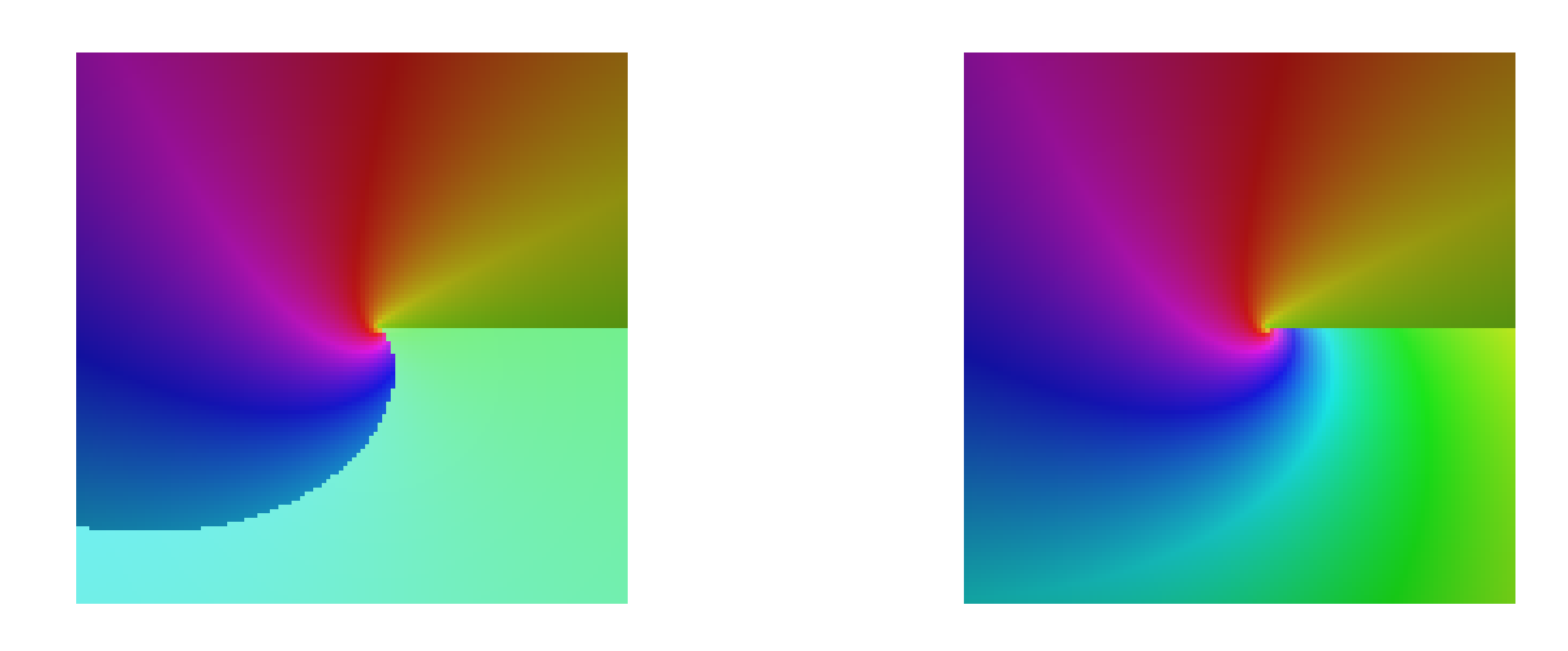
Unfortunately, when subjecting it to randomized testing, I found out that these formulas are all incorrect! Here is the problem: with complex parameters, the branch cuts induced by taking the principal branch of $\Gamma(1-s, -a \log(z))$ or $\Gamma(1-s, -(a+1/2) \log(z))$ are not the ones we want for the Lerch transcendent.
The bug is illustrated in the following domain coloring plot of $\Phi(z, 1-i, 1+i)$. On the left is the incorrect Lerch transcendent (note the spurious branch cut in the lower plane) as computed by mpmath's lerchphi and on the right is the correct version computed by lerch_hankel:
Here is an explicit numerical example showcasing the bug in mpmath:
>>> print(lerchphi(-8j, 1-1j, 1+1j))        # WRONG
(-68.7248098321797 + 18.3615875253618j)

>>> print(lerch_hankel(-8j, 1-1j, 1+1j))     # CORRECT
(-0.187147647099947 + 0.0313275836315882j)
Mathematica gets it right:
In[1]:= N[HurwitzLerchPhi[-8 I, 1-I, 1+I], 15]

Out[1]= -0.187147647099946+0.031327583631588 I
The implementation of the Lerch transcendent now in Arb, which uses the Laplace transform integral instead of the Abel-Plana formula, gets it right (here using a wrapper placed in Python-FLINT):
>>> from flint import *

>>> acb(-8j).lerch_phi(1-1j, 1+1j)
[-0.1871476470999 +/- 5.62e-14] + [0.0313275836316 +/- 2.31e-14]j

>>> ctx.dps = 30
>>> acb(-8j).lerch_phi(1-1j, 1+1j)
[-0.1871476470999464791803420189 +/- 5.42e-29] + [0.0313275836315882418015026098 +/- 1.24e-29]j
It would be nice to have a corrected version of the Abel-Plana formula, because in my experiments it is about twice as fast as the Laplace transform representation. I think one way to fix it is to use a Hankel contour representation of the incomplete gamma function, but then there is probably no advantage over using the Hankel integral for the Lerch transcendent directly.
Some timings
Here are timings to compute a few different values with the old Lerch transcendent implementation in mpmath and the new implementation in Arb (I used 3.333 * d + 10 bits of precision to get roughly $d$ digits with Arb):
| Value | Digits | mpmath lerchphi | Arb acb_dirichlet_lerch_phi |
|---|---|---|---|
| $\Phi(0.75, 0.75, 0.75)$ ($|z| < 1$, real) |
10 | 0.00987 s | 0.000124 s |
| 100 | 0.223 s | 0.00247 s | |
| 1000 | 28.3 s | 0.865 s | |
| $\Phi(0.5+0.5i, 0.5+0.5i, 0.25+0.75i)$ ($|z| < 1$, complex) |
10 | 0.0784 s | 0.000323 s |
| 100 | 0.754 s | 0.000538 s | |
| 1000 | 73.0 s | 1.516 s | |
| $\Phi(-2, 0.75, 0.75)$ ($|z| > 1$, real) |
10 | 0.0325 s | 0.000807 s |
| 100 | 0.604 s | 0.0154 s | |
| 1000 | 31.2 s | 4.306 s | |
| $\Phi(1+2i, 0.5+0.5i, 0.25+0.75i)$ ($|z| > 1$, complex) |
10 | 0.0266 s | 0.00222 s |
| 100 | 0.877 s | 0.0409 s | |
| 1000 | 63.7 s | 10.438 s |
Here are enclosures computed by Arb:
[2.4530308232 +/- 2.46e-11]
[2.4530308231{...80 digits...}4294101340 +/- 2.62e-101]
[2.4530308231{...982 digits...}0801442123 +/- 1.99e-1003]

[2.567366619838 +/- 8.21e-13] + [-0.2104839969647 +/- 7.41e-14]*I
[2.5673666198{...82 digits...}0617104976 +/- 6.47e-103] + [-0.2104839969{...83 digits...}2656088048 +/- 5.29e-104]*I
[2.5673666198{...984 digits...}5510822666 +/- 5.32e-1005] + [-0.2104839969{...985 digits...}8391518638 +/- 4.07e-1006]*I

[0.6709167646 +/- 7.39e-11]
[0.6709167645{...79 digits...}6621886305 +/- 1.93e-100]
[0.6709167645{...982 digits...}6552381516 +/- 6.64e-1003]

[1.1885421054 +/- 6.97e-11] + [0.600280289 +/- 2.33e-10]*I
[1.1885421054{...80 digits...}5262646586 +/- 6.70e-101] + [0.6002802888{...79 digits...}1836025011 +/- 1.06e-100]*I
[1.1885421054{...982 digits...}3427814955 +/- 3.63e-1003] + [0.6002802888{...982 digits...}9230553496 +/- 7.21e-1003]*I
Arb's performance is neither terrible nor particularly impressive. It is much faster than mpmath, but that is not a high bar; it would be worthwhile to improve the implementations in both libraries. (I should at the very least fix mpmath so that it computes the function correctly...)
It is worth noting that the Lerch transcendent in Arb checks for some special cases, so if you for example evaluate $\Phi(1,s,1)$, it will fall back on the fast code for the Riemann zeta function instead of using the much slower general-purpose Lerch transcendent code.
Other algorithms
Euler-Maclaurin summation and asymptotic expansions
There are various asymptotic expansions of Lerch transcendent with respect to $z$, $s$ or $a$; the Euler-Maclaurin formula can also be used in some cases. Such methods are only applicable for parameters in certain ranges, but they will be much more efficient than numerical integration when they do apply. Some algorithms (and implementation results) can be found in a nice preprint by Guillermo Navas-Palencia and in his PhD thesis. It would be a lot of work to implement these methods properly in Arb (along with good heuristics to choose between them) but it can certainly be done.
Erdélyi series
A useful representation for $|\log(z)| < 2 \pi$ is $$\Phi(z,s,a)=z^{-a}\left[\Gamma(1-s)\left(-\log (z)\right)^{s-1} +\sum_{k=0}^\infty \zeta(s-k,a)\frac{\log^k (z)}{k!}\right]$$ which seems to be known as the "Erdélyi series". This series is especially nice near $z = 1$ where $|\log(z)|$ is small. I did not implement this formula as I do not have an explicit bound for the truncation error valid for complex $s$ (working out such a bound is certainly doable, but will require a bit of calculation). Also, evaluating the Hurwitz zeta function values $\zeta(s-k,a)$ is going to be slow in general; to make it really efficient, some kind of multi-evaluation algorithm is needed.
When $s = n$ is a positive integer, the limiting version of the Erdélyi series is $$\Phi(z,n,a)=z^{-a}\left\{ \sum_{{k=0}\atop k\neq n-1}^ \infty \zeta(n-k,a)\frac{\log^k (z)}{k!} +\left[\psi(n)-\psi(a)-\log(-\log(z))\right]\frac{\log^{n-1}(z)}{(n-1)!} \right\}$$ and here things are a bit nicer since $\zeta(n-k,a)$ reduces to a Bernoulli polynomial when $k \ge n$. The Bernoulli polynomials can be computed quite cheaply using the defining exponential generating function, and we can also get bounds easily here. By a quick calculation, Bernoulli numbers satisfy $$|B_n| \le \frac{\pi^2}{3} \frac{n!}{(2\pi)^n}$$ and Bernoulli polynomials satisfy $$|B_n(x)| = \left| \sum_{k=0}^n {n \choose k} B_k x^{n-k} \right| \le \frac{\pi^2}{3} \sum_{k=0}^n {n \choose k} \frac{(n-k)!}{(2\pi)^{n-k}} |x|^k \le \frac{\pi^2}{3} \frac{n!}{(2\pi)^{n}} \sum_{k=0}^n \frac{(2 \pi |x|)^k}{k!} \le \frac{\pi^2}{3} \frac{n!}{(2\pi)^{n}} e^{2 \pi |x|}.$$ Writing the Bernoulli polynomial part of the Erdélyi series as $$\sum_{k=0}^{\infty} -\frac{B_{k+1}(a)}{k+1} \frac{\log^{n+k}(z)}{(n+k)!}$$ the tail should be bounded (modulo errors in my calculations) by $$\sum_{k=K}^{\infty} \le \frac{\pi^2}{3} e^{2\pi|a|} \frac{1}{(2 \pi)^K} \frac{K!}{(K+n)!} \frac{|\log(z)|^{K+n}}{(2 \pi - |\log(z)|)}.$$ I did not implement this formula in Arb, but I might do so in the near future.
Approximate functional equation
Another very interesting approach is a version of the "approximate functional equation" technique for the Riemann zeta function. This algorithm for the Lerch transcendent was developed by Richard Crandall (Algorithm 3 in the Bailey and Borwein reference), who calls it a "Riemann-splitting algorithm". A naive mpmath implementation is given below:
from mpmath import *

def S(z):
    return sign(re(z))

def lerch_crandall(z,s,a):
    z = mpmathify(z)
    s = mpmathify(s)
    a = mpmathify(a)
    res = 0
    l = +pi
    if isint(a):
        res -= z**(-a) * l**(s/2) / s * rgamma(s/2)
    if z == 1:
        res += 1/(s-1) * pi**0.5 * l**((s-1)/2) * rgamma(s/2)
    def f(n):
        A = n + a
        return z**n / (A**2)**(s/2) * (gammainc(s/2, l*A**2)*rgamma(s/2) + gammainc((s+1)/2, l*A**2)*rgamma((s+1)/2) * S(A))
    res += 0.5 * nsum(f, [-inf,inf], method="d")
    def g(u):
        U = u + log(z)/(2*pi*1j)
        return exp(-2*pi*1j*a*u)/((U**2)**((1-s)/2)) * (gammainc((1-s)/2, pi**2*U**2/l)*rgamma(s/2) + 1j*gammainc(1-s/2, pi**2*U**2/l)*rgamma((s+1)/2)*S(U))
    res += pi**(s-0.5) / (2*z**a) * nsum(g, [-inf,inf], method="d")
    return res

z, s, a = 2+3j, 1-2j, 0.75-0.5j
mp.dps = 30
mp.pretty = True
print(lerch_crandall(z,s,a))
print(lerchphi(z,s,a))
With proper optimizations, I believe this could be one of the most efficient ways to evaluate the analytic continuation of the Lerch transcendent. However, one would have to work out error bounds and check validity for different complex parameters; there are certainly some branch cut issues that need to be resolved.
References
- Karim Belabas and Henri Cohen (2021). Numerical Algorithms for Number Theory Using Pari/GP. AMS.
- A. Erdélyi, W. Magnus, F. Oberhettinger, and F. G. Tricomi (1953). Higher Transcendental Functions. Vol. I. McGraw-Hill.
- NIST Digital Library of Mathematical Functions. https://dlmf.nist.gov/25.14.
- Guillermo Navas-Palencia (2019). Numerical methods and arbitrary-precision computation of the Lerch transcendent. Preprint. https://gnpalencia.org/research/GNP_Lerch_2018.pdf.
- D. H. Bailey and J. M. Borwein (2015). Crandall's computation of the incomplete Gamma function and the Hurwitz Zeta function, with applications to Dirichlet L-series. Applied Mathematics and Computation 268. 462–477. https://www.davidhbailey.com/dhbpapers/lerch.pdf
- R. Crandall (2012). Unified algorithms for polylogarithm, L-series, and zeta variants, In Algorithmic Reflections: Selected Works. PSIpress.
fredrikj.net |
Blog index |
 RSS feed |
Follow me on Mastodon |
Become a sponsor
RSS feed |
Follow me on Mastodon |
Become a sponsor