Arb 2.13.0 released, and more on integration

February 28, 2018

I issued version 2.13 of Arb just a few days ago. As usual, downloads are available via GitHub, and there is an extensive changelog in the documentation. This release contains few major new features, but there are many significant optimizations, one important bug fix, and various build system and compatibility fixes. More detail on some of the improvements follows below.

Sage interface, and papers

First, some related announcements. A Sage wrapper for the rigorous numerical integration code in Arb has been written by Marc Mezzarobba and Vincent Delecroix. The feature was recently merged into the development branch of Sage, and should be available in the next release. One can now do this:

sage: C = ComplexBallField(333)
sage: C.integral(lambda x, _: sin(x+exp(x)), 0, 8)
[0.34740017265724780787951215911989312465745625486618018388549271361674821398878532052968510434660 +/- 5.97e-96]

The second parameter passed to the integrand is a flag to test analyticity, which can be ignored for meromorphic integrands but must be handled by the user when integrating functions with branch cuts. Here is an example from the documentation:

sage: def my_sqrt(z, analytic):
....:     if (analytic and not z.real() > 0
....:                  and z.imag().contains_zero()):
....:         return CBF(NaN)
....:     else:
....:         return z.sqrt()
sage: CBF.integral(my_sqrt, -1 + CBF(i), -1 - CBF(i))
[+/- 1.14e-14] + [-0.4752076627926 +/- 5.18e-14]*I

Another ticket is currently in progress which will add an analytic keyword argument to many basic functions, so that the example above can be written more simply as:

sage: CBF.integral(lambda z, d: z.sqrt(analytic=d), -1 + CBF(i), -1 - CBF(i))
[+/- 1.14e-14] + [-0.4752076627926 +/- 5.18e-14]*I

For readers who are interested in how the integration code in Arb works, two papers are now available:

https://arxiv.org/abs/1802.07942 (Numerical integration in arbitrary-precision ball arithmetic)
https://arxiv.org/abs/1802.03948 (Fast and rigorous arbitrary-precision computation of Gauss-Legendre quadrature nodes and weights; coauthored with Marc Mezzarobba)

Tighter bounds

The most important change in Arb 2.13 is that the functions arb_div, arb_sqrt, arb_rsqrt, arb_exp, arb_log and arb_atan have been optimized for wide input (roughly when the relative error is larger than $2^{-20} \approx 10^{-6}$). In most cases, these functions now compute balls that are nearly the smallest possible for such input, and they handle this case faster than the previous code did. The functions acb_log and acb_rsqrt have also been improved for wide intervals, as well as Airy functions and gamma functions, although not to the same extent.

This plot of the real part of $\log(x+0.2i)$ evaluated on wide balls gives an example of the improvement (Arb 2.12 on the left, Arb 2.13 on the right):

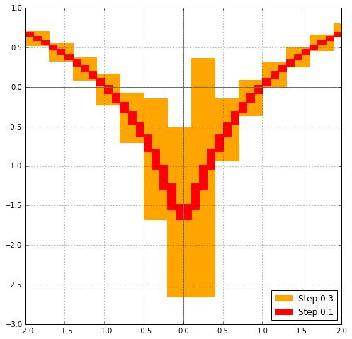
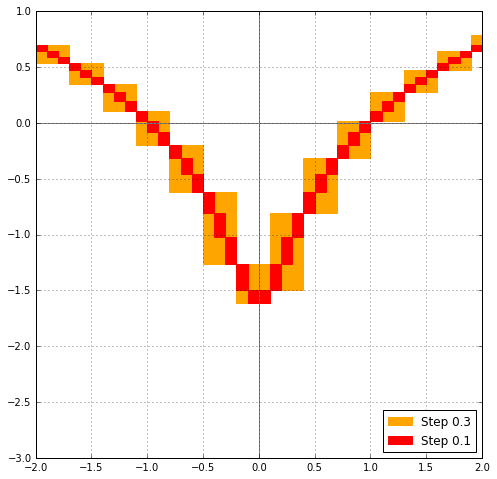
In particular, the new implementations of arb_rsqrt, arb_log, acb_rsqrt and acb_log now avoid returning non-finite intervals for wide input close to (but not touching) zero. For example, $\log([1 \pm 0.5] + [1 \pm 0.5] i)$ previously gave $\operatorname{NaN} + \operatorname{NaN} i$, but now gives $$[0.202732554\ldots \pm 0.550] + [0.785398161\ldots \pm 0.464] i.$$

More generally, the new versions of arb_div, arb_sqrt, arb_rsqrt, arb_exp, arb_log and arb_atan take the accuracy of the input into account when setting the internal working precision. For example, if the user evaluates $\exp([1 \pm 2^{-128}])$ at $1024$ bits of precision, Arb would previously compute $\exp(1)$ to 1024 bits of precision; it now recognizes that only about 128 bits are meaningful in the output and automatically uses just slightly more than 128 bits internally.

In the future, similar improvements will be made to trigonometric and other transcendental functions. Also basic arithmetic (addition and multiplication) should be optimized later, but this is a significantly harder project since it requires extensive low-level coding.

The improvements for wide input are useful in many situations, but one of the immediate applications is to speed up numerical integration. For example, compared to the timings in the first blog post, $\int_1^{1+1000i} \Gamma(x) dx$ is now about five times faster and $\int_0^1 -\log(x) / (1+x) dx$ is about three times faster.

Another nice test integral (included as a benchmark problem in the paper) is $\int_0^{\infty} e^{-x} \operatorname{Ai}(-x) dx$, which now is fast due to improvements to Airy functions. As a reminder, the integration code in Arb does not support infinite intervals directly, so the actual computation is $\int_0^N e^{-x} \operatorname{Ai}(-x) dx + [\pm 2^{-p}]$ with $N = \lceil p \log(2) \rceil$. Using examples/integrals.c:

$ build/examples/integrals -i 30 -prec 64
I30 = int_0^{inf} exp(-x) Ai(-x) dx   (using domain truncation) ...
cpu/wall(s): 0.027 0.027
I30 = [0.37875160537908653 +/- 5.88e-18]

$ build/examples/integrals -i 30 -prec 333
I30 = int_0^{inf} exp(-x) Ai(-x) dx   (using domain truncation) ...
cpu/wall(s): 1.023 1.023
I30 = [0.37875160537908653500019243447885263024846209695031040896622107141190757271988163631327321306434417 +/- 5.69e-99]

$ build/examples/integrals -i 30 -prec 1000
I30 = int_0^{inf} exp(-x) Ai(-x) dx   (using domain truncation) ...
cpu/wall(s): 16.702 16.703
I30 = [0.37875160537908653500019243447885263024846209695031040896622107141190757271988163631327321306434416621461318532802401368947062052673149354464779312503421623265364558051520769109402014170252004204400705508626352742889810144000765626119328682493574429257398097397998070965416640375832244959500557980129 +/- 9.56e-300]

This integral is about 20 times faster in Arb than in mpmath.

New convenience functions

Some new convenience functions for numerical integration have been added in Arb 2.13. These include acb_real_abs, acb_real_sgn, acb_real_heaviside, acb_real_floor, acb_real_ceil, acb_real_min, acb_real_max which implement the piecewise analytic real functions $|x|$, $\operatorname{sgn}(x)$, $H(x)$, $\lfloor x \rfloor$, $\lceil x \rceil$, $\min(x,y)$, $\max(x,y)$ extended to piecewise complex analytic functions. These builtin methods make it easy to integrate typical discontinuous or piecewise-defined real functions.

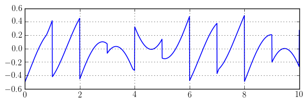
The following C code (also available in examples/integrals.c) defines $f(x) = (x-\lfloor x \rfloor - \tfrac{1}{2}) \max(\sin(x), \cos(x))$:

int f(acb_ptr res, const acb_t z, void * param, slong order, slong prec)
{
    acb_t s, t;
    acb_init(s);
    acb_init(t);
    acb_real_floor(res, z, order != 0, prec);
    if (acb_is_finite(res))
    {
        acb_sub(res, z, res, prec);
        acb_set_d(t, 0.5);
        acb_sub(res, res, t, prec);
        acb_sin_cos(s, t, z, prec);
        acb_real_max(s, s, t, order != 0, prec);
        acb_mul(res, res, s, prec);
    }
    acb_clear(s);
    acb_clear(t);
    return 0;
}

One of the benchmark problems in the paper is to compute $\int_0^{10} f(x) dx$. The integrand looks like this:

Sample output:

$ build/examples/integrals -i 27 -prec 64
I27 = int_0^10 (x-floor(x)-1/2) max(sin(x),cos(x)) dx ...
cpu/wall(s): 0.037 0.037
I27 = [-0.1428186420263281 +/- 6.67e-17]

$ build/examples/integrals -i 27 -prec 333
I27 = int_0^10 (x-floor(x)-1/2) max(sin(x),cos(x)) dx ...
cpu/wall(s): 1.415 1.415
I27 = [-0.142818642026328083760191649507947165066535747959413237185490975194164859231025185646415489051416 +/- 5.08e-97]

fredrikj.net | Blog index | RSS feed | Follow me on Mastodon | Become a sponsor