fredrikj.net / blog /

Interesting interference integrals

July 12, 2018

Chapter 36 of the NIST Digital Library of Mathematical Functions covers a class of lesser-known special functions called "diffraction catastrophe integrals". These functions describe complex wave interference phenomena such as the diffraction patterns of optical caustics. The visualizations section has some neat graphics that would be nice to replicate!

Essentially, diffraction catastrophe integrals $\Psi(x_1,\ldots,x_n)$ are oscillatory integrals of the form $\int_{-\infty}^{\infty} \exp(i \Phi(t)) dt$ or $\int_{-\infty}^{\infty} \int_{-\infty}^{\infty} \exp(i \Phi(s,t)) ds dt$ for certain families of polynomials $\Phi$ whose coefficients depend on the parameters $x_1,\ldots,x_n$. The word "catastrophe" comes from catastrophe theory and signifies that the behavior of such functions can change suddenly and dramatically with a small change in the parameters. The simplest example is the Airy function $\int_{-\infty}^{\infty} e^{i (t^3 + x t)} dt = \pi 3^{-1/3} \operatorname{Ai}(3^{-1/3} x)$, which has a turning point at $x = 0$ where the behavior changes from oscillatory to exponentially decreasing. The general catastrophe integrals can be thought of as multivariate, higher-degree generalizations of Airy functions.

The first example that is not representable in terms of classical special functions such as Airy functions is the Pearcey integral $$P(x,y) = \int_{-\infty}^\infty \exp(i(t^4+x t^2+y t)) \, dt.$$ This looks like an interesting challenge for the rigorous numerical integration code in Arb. Of course, the plan is not to integrate directly along the real line which is nearly hopeless numerically (at least without the use of special convergence acceleration methods for oscillatory integrals). Instead, we rotate the path by an angle $\exp(\pi i / 8)$ to obtain (Connor and Farrelly, 1981) the exponentially decaying integral $$P(x,y) = 2 \exp(\pi i / 8) \int_0^{\infty} \exp(-t^4 + a t^2) \cosh(b t) dt$$ where $a = \exp(3 \pi i / 4) x$ and $b = \exp(5 \pi i / 8) y$.

The integration code in Arb requires a finite interval, so we truncate the path at some point $N \ge 1$. The truncation error is bounded by $$\int_N^{\infty} \exp(-t^4 + A t^2 + B t) dt = \int_N^{\infty} \exp(-t^4 (1 - A / t^2 - B / t^3)) dt \le \int_N^{\infty} \exp(-C t^4 ) dt \le \frac{\exp(-C N^4 )}{C}$$ where $A = \max(0,\operatorname{Re}(a))$, $B = |\operatorname{Re}(b)|$ and $C = 1 - A / N^2 - B / N^3$, provided that $C > 0$.

I wrote a quick implementation of the function and put the code into a copy of the Arb example program complex_plot.c to be able to draw pictures. I don't plan to add the Pearcey integral to Arb itself yet, but I've made the code available as a gist file for now.

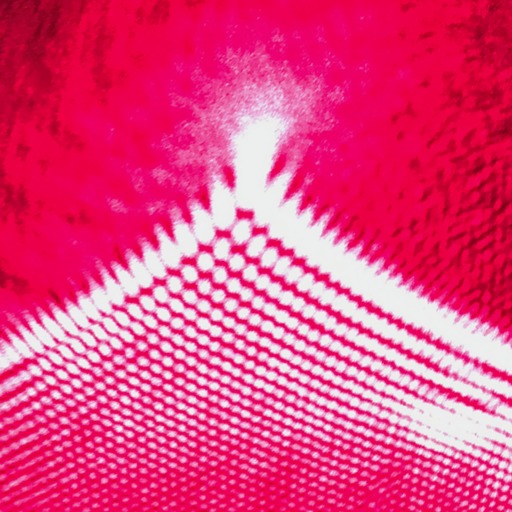
The left image below is the output of ./a.out -size 512 512 -range -12.5 12.5 -20 5 -color 4. This shows $P(y,x)$ for $-12.5 \le x \le 12.5$ and $-20 \le y \le 5$. Note that I have swapped the $x$ and $y$ coordinates, because this is how the function is rendered in all the other visualizations I have seen.

The right image below is "a photograph of a cusp caustic produced by illuminating a flat surface with a laser beam through a droplet of water" taken from the Wikipedia page for the Pearcey integral (CC-BY-SA, Dan Piponi).

This 512 by 512 pixel image takes 15 minutes to render. In other words, Arb manages 300 evaluations of the function per second on average over this range. On the domain $|x|, |y| \le 5$, Arb manages 1600 evaluations per second; the evaluation is significantly slower for larger negative $y$ since larger cancellations appear in the integral. The complex_plot code starts with 30 bits of precision and doubles the precision until convergence; near the bottom where $y = -20$, it converges at 120 bits.

In a recent question on the Mathematica Stack Exchange, Emilio Pisanty asks for a Mathematica implementation of the diffraction catastrophe integrals. He is skeptical about a straightforward implementation using Mathematica's NIntegrate:

I'm a bit wary of the numerical integrations, particularly as you go to the $y \ll -1$ region and the integrals get very oscillatory - I've found the simpler NIntegrate implementations to suddenly go belly-up. (...) Well, I'm running those same plots down to $y = -18$ and it's already complaining about NIntegrate::ncvi.

With the Arb integration code and a simple precision-doubling strategy, we get an implementation that is reliable and reasonably efficient. It should also be noted that it works with complex values of the parameters $x$ and $y$ if needed.

Of course, it must be stressed that this is a brute force solution to compute the Pearcey integral, and a much better implementation is possible. The performance with large parameters could be improved substantially by deforming the contour to try to bypass the cancellation problems (Kirk, Connor and Hobbs, 2000). The integration strategy could also be complemented with use of Taylor and asymptotic expansions (Lopez and Pagola, 2016).

As noted above, I have not yet added the Pearcey integral to Arb itself since it is a rather obscure function. A more substantial project would be to implement the complete suite of diffraction catastrophe integrals from DLMF chapter 36 (and to optimize the implementation a bit more). I will probably not have time to work on this myself, but if anyone is interested in working on it, please let me know.

The Pearcey integral was introduced by T. Pearcey in a 1946 paper. In this paper, we find the following impressive hand-drawn magnitude and phase plots:

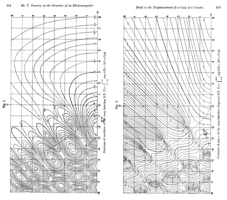
Pearcey explains how the figures were created:

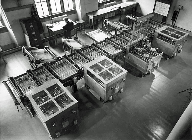
The integral part of the expression (2), of which figs. 1 and 2 represent the modulus and phase respectively in terms of the cartesion co-ordinates $X$ and $Y$, was computed in a series of steps. First, tables of the $\tfrac{1}{4}$-order Bessel functions were used for the evaluation of $I(X, 0)$ and $\left[\frac{\partial^2 I(X,Y)}{\partial Y^2}\right]_{Y=0}$ From a pair of differential equations satisfied by $I(X, Y)$, the function was evaluated along a number of lines lying parallel to the $Y$-axis by use of the Cambridge differential analyser. In the regions where the analyser was incapable of giving a sufficiently accurate solution the function was evaluated from its power series and its appropriate asymptotic expansions.

Here is a picture of the Cambridge differential analyser (CC-BY, University of Cambridge):

The mind boggles!

fredrikj.net  |  Blog index  |  RSS feed  |  Follow me on Mastodon  |  Become a sponsor