fredrikj.net / blog /
Arb 2.10.0 released
February 27, 2017
Arb version 2.10.0, available today, brings new elliptic functions and integrals, improvements to basic complex arithmetic, a new implementation of the dilogarithm function, reduced library size, and more.
More and improved elliptic functions and integrals
Elliptic functions and elliptic integrals are a frequently requested feature (physicists love them). The complete elliptic integrals of first and second kind $K(m)$ and $E(m)$ as well as the Weierstrass elliptic function $\wp(z)$ (together with its derivatives) have been available for some time (see the earlier writeup about elliptic functons). Arb 2.10 adds several functions:
- The complete elliptic integral of the third kind $\Pi(n,m)$.
- The incomplete elliptic integrals $F(\phi,m)$, $E(\phi,m)$ and $\Pi(n,\phi,m)$.
- Carlson's symmetric forms of incomplete elliptic integrals $R_F(x,y,z)$, $R_C(x,y)$, $R_G(x,y,z)$, $R_J(x,y,z,p)$ and $R_D(x,y,z)$.
- The inverse Weierstrass elliptic function, $\wp^{-1}(z)$ (this is equivalent to an incomplete elliptic integral).
- The Weierstrass zeta and sigma functions $\zeta(z)$ and $\sigma(z)$.
- Utility functions for computing the Weierstrass invariants and lattice roots.
All the various elliptic functions and integrals have been placed in a module of their own: acb_elliptic.h.
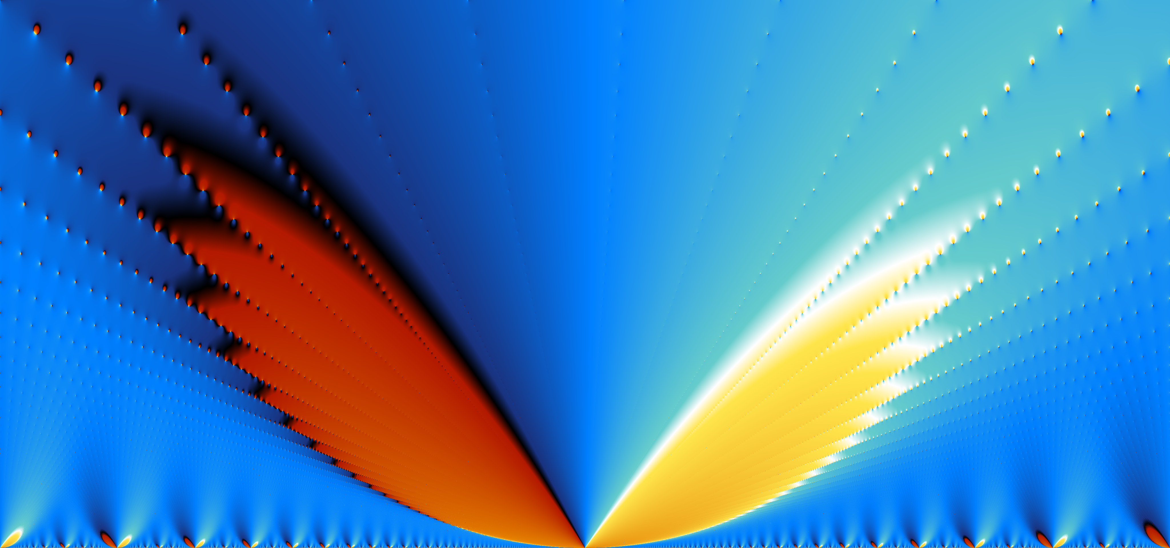
Elliptic functions make for striking pictures. Consider this plot of the phase of the Weierstrass zeta-function $\zeta(0.25 + 2.25i)$ as the lattice parameter $\tau$ varies over $[-0.25,0.25] + [0,0.15]i$. Wings spread along the infinitely many rays of poles and zeros! Click the image for a 4096x1920 pixel version.
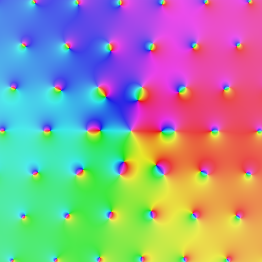
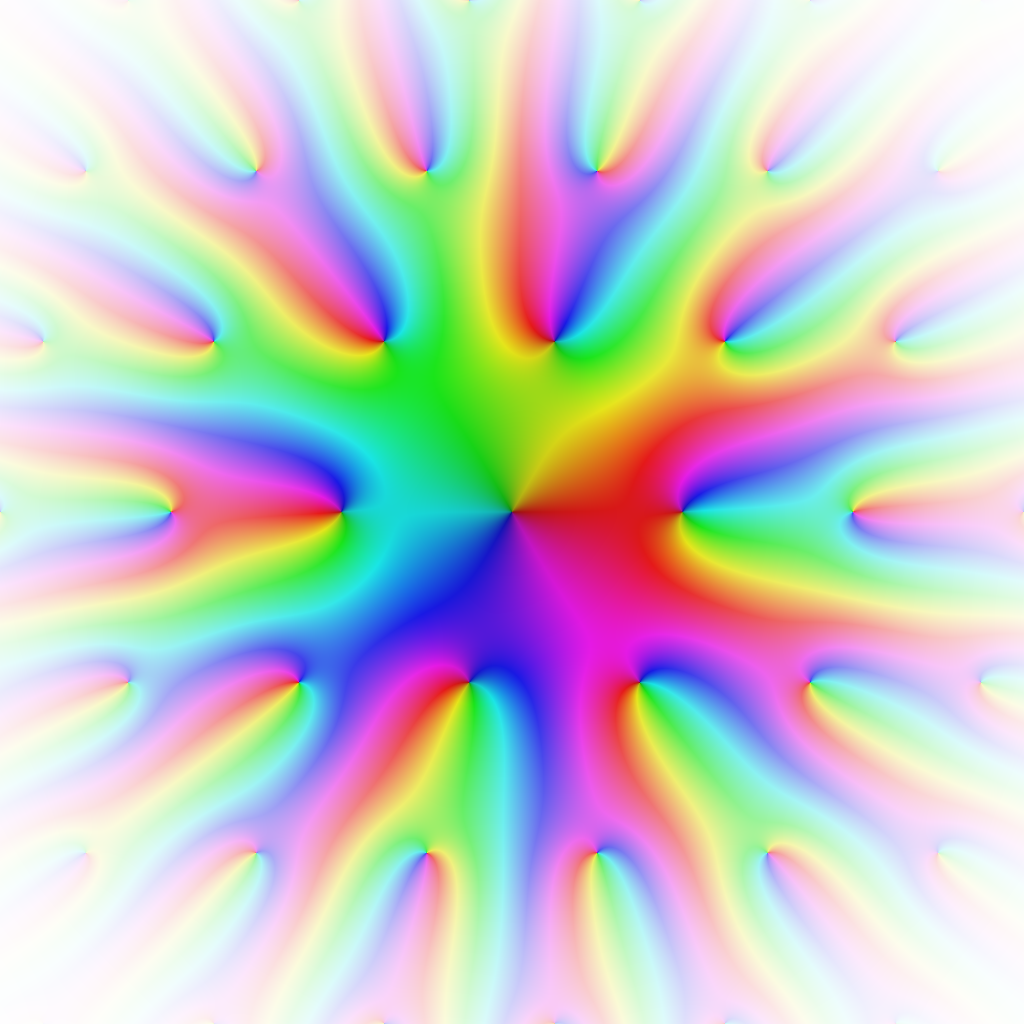
Two electric domain coloring plots, of $\zeta(z)$ and $\sigma(z)$ on the lattice generated by $1$ and $\tau = 0.25+i$ (slightly higher resolution available by clicking the images):
The Weierstrass zeta and sigma functions (as well as $\wp'(z)$) are computed via derivatives of Jacobi theta functions, which were already available. However, an important improvement was necessary: previously, Arb applied modular transformations to the lattice parameter $\tau$ to bring it to the fundamental domain when computing theta functions, but it did not do so for the derivatives. This meant that $\tau$ with small imaginary parts were very inefficient when computing derivatives. This has now been fixed in Arb 2.10. (There are still improvements to be done, including using quasiperiod reductions for large $z$ and finding some symbolic simplifications to avoid divisions of large exponentials.)
Concerning incomplete elliptic integrals, much of what I wrote about their implementation in mpmath almost seven years ago (time flies) still applies. I chose to use the Carlson symmetric forms as the building blocks just like in mpmath since Carlson gives convenient algorithms and the functions behave well with complex arguments. See Carlson's paper Numerical computation of real or complex elliptic integrals (arXiv copy) and the DLMF chapter on elliptic integrals. The Legendre forms have very ugly branch cut structure, so it makes more sense to compute them from the Carlson forms than vice versa.
I will sketch the algorithm in one case. To compute $$R_F(x,y,z) = \frac{1}{2} \int_0^{\infty} \frac{dt}{\sqrt{(t+x)(t+y)(t+z)}}$$ one repeatedly performs a "duplication step" which replaces $x,y,z$ by $(x+\lambda)/4$, $(y+\lambda)/4$, $(z+\lambda)/4$ where $\lambda = \sqrt{x} \sqrt{y} + \sqrt{x} \sqrt{z} + \sqrt{y} \sqrt{z}$. Each duplication step brings the arguments closer to each other by a factor four, and when the arguments are close enough, say within $\epsilon$ of each other, $R_F(x,y,z)$ can be approximated by a multivariate Taylor series. (This series is a multivariate hypergeometric series.) In Arb, a hardcoded Taylor polynomial of total degree 7 is used, so the error is of order $\epsilon^8$ (it is not too hard to prove an explicit bound that can be used in interval arithmetic). Each duplication step thus gives $8 \cdot 2 = 16$ bits of accuracy. This is reasonably efficient, which is quite nice considering the simplicity of the algorithm (though one could still do better for very high precision).
The following table compares the time to compute $R_F(x,y,z)$ with mpmath (in SageMath) and Arb 2.10, first for real arguments $x = 2, y = 3, z = 5$ and second for complex arguments $x=2+i, y=-3+2i, z=5-i$. There are no big surprises: both implementations have similar scaling, but the arithmetic in Arb is a lot faster (with an order of magnitude difference at machine precision).
| prec (bits) | mpmath real |
Arb 2.10 real |
mpmath complex |
Arb 2.10 complex |
|---|---|---|---|---|
| 53 | 0.000092 | 0.0000094 | 0.00021 | 0.000025 |
| 333 | 0.00033 | 0.000059 | 0.00086 | 0.00019 |
| 3333 | 0.0079 | 0.0024 | 0.031 | 0.011 |
| 33,333 | 1.6 | 0.62 | 8.1 | 2.5 |
| 333,333 | 190 | 685 |
The numerical intervals computed by Arb in the real case are:
[0.559406346700304 +/- 7.77e-16]
[0.5594063467{...79 digits...}3918527992 +/- 6.32e-100]
[0.5594063467{...982 digits...}7659941906 +/- 4.79e-1003]
[0.5594063467{...10013 digits...}5933378605 +/- 7.43e-10034]
[0.5594063467{...100322 digits...}0322455428 +/- 5.27e-100343]
In the complex case:
[0.554584622469726 +/- 8.90e-16] + [-0.269015812212692 +/- 9.00e-16]*I
[0.5545846224{...79 digits...}0470193768 +/- 9.14e-100] + [-0.2690158122{...79 digits...}0721042230 +/- 7.71e-100]*I
[0.5545846224{...934 digits...}7564768151 +/- 8.21e-955] + [-0.2690158122{...934 digits...}9779878557 +/- 6.80e-955]*I
[0.5545846224{...9480 digits...}2190805743 +/- 2.92e-9501] + [-0.2690158122{...9481 digits...}0850324130 +/- 8.29e-9502]*I
[0.5545846224{...94944 digits...}2549266389 +/- 2.97e-94965] + [-0.2690158122{...94944 digits...}8882734112 +/- 1.04e-94965]*I
Some precision is lost at high precision with complex arguments. This is due to overestimation when doing complex interval arithmetic, which can lead errors to build up rapidly when performing an iteration of the type $x_k = f(x_{k-1})$ (the duplication step in Carlson's algorithm). This problem could be fixed with a bit of work. It's not too bad currently, because we only lose a few percent of the significant digits, but it would be nice to preserve full accuracy. The situation could actually have been much worse (see the next section).
More accurate division and square roots of complex numbers
Arb performs the complex division $z / w$ as $z \cdot w^{-1}$ (except in special cases, e.g. when $w$ is pure real or imaginary). Previously, Arb would compute the reciprocal of a complex number naively using the formula $$\frac{1}{a+bi} = \frac{a}{a^2 + b^2} - \frac{i b}{a^2 + b^2}.$$ The problem with using this formula is that it inflates the error bounds in interval arithmetic (due to the dependency of errors between the numerator and denominator which does not cancel out). In fact, the way it was implemented before, the interval computed for $a^2 + b^2$ could contain zero even if $a$ or $b$ certainly was nonzero, leading to a spurious division by zero. Arb is now smarter: it evaluates the reciprocal formula only at the midpoints of the intervals, and then computes a more accurate error bound for the real and imaginary parts separately. A side effect is that $w^{-1}$ certainly will be finite if $w$ does not contain zero. The following examples show the the improvement in accuracy. Here, the input is set with arb_set_str and the output is printed with acb_printn, so the actual bounds before the binary-decimal conversion are smaller than the printed values.
Input:    [3 +/- 1e-14] + [5 +/- 1e-13]*I
Arb 2.9:  [0.08823529411765 +/- 6.01e-15] + [-0.14705882352941 +/- 9.30e-15]*I
Arb 2.10: [0.08823529411765 +/- 5.78e-15] + [-0.14705882352941 +/- 4.20e-15]*I

Input:    [3 +/- 0.1] + [5 +/- 0.1]*I
Arb 2.9:  [0.09 +/- 9.27e-3] + [-0.1 +/- 0.0576]*I
Arb 2.10: [0.09 +/- 6.81e-3] + [-0.15 +/- 8.03e-3]*I

Input:    [3 +/- 1.0] + [5 +/- 1.0]*I
Arb 2.9:  [+/- 0.251] + [+/- 0.376]*I
Arb 2.10: [+/- 0.178] + [+/- 0.243]*I

Input:    [3 +/- 2.999] + [5 +/- 4.999]*I
Arb 2.9:  [+/- inf] + [+/- inf]*I
Arb 2.10: [+/- 4.81e+6] + [+/- 5.66e+6]*I
As another illustration, we set $z_0 = 3+5i$ and compute the sequence $z_{k} = 1 / z_{k-1}$. Although $z_{k+2} = z_k$ in exact arithmetic, each iteration gives slightly larger errors in interval arithmetic. Eventually $z_{k-1}$ might contain zero so that $z_k$ blows up, depending on how the interval arithmetic is implemented. With Arb's representation of intervals, the division by zero is in fact unavoidable (unless $z_0$ is set to a number with an exact inverse), but we can at least hope to postpone it as far as possible. With the old code, blowup happens at $k = 34$ at 53-bit precision. With the new code, the division by zero does not occur until $k = 72$. The following printout shows the significant digits as computed with the old and the new division and printed with acb_printn(x, 20, ARB_STR_NO_RADIUS):
k   Arb 2.9                                     Arb 2.10
-----------------------------------------------------------------------------------------
1   0.0882352941176471 - 0.1470588235294117*I   0.0882352941176471 - 0.1470588235294117*I
2   3.00000000000000 + 5.00000000000000*I       3.00000000000000 + 5.00000000000000*I
3   0.088235294117647 - 0.147058823529412*I     0.088235294117647 - 0.147058823529412*I
4   3.0000000000000 + 5.0000000000000*I         3.0000000000000 + 5.0000000000000*I
5   0.08823529411765 - 0.14705882352941*I       0.088235294117647 - 0.147058823529412*I
6   3.000000000000 + 5.000000000000*I           3.0000000000000 + 5.0000000000000*I
7   0.0882352941176 - 0.1470588235294*I         0.08823529411765 - 0.14705882352941*I
8   3.00000000000 + 5.00000000000*I             3.0000000000000 + 5.0000000000000*I
9   0.088235294118 - 0.147058823529*I           0.08823529411765 - 0.14705882352941*I
10  3.0000000000 + 5.0000000000*I               3.000000000000 + 5.000000000000*I
11  0.08823529412 - 0.14705882353*I             0.0882352941176 - 0.1470588235294*I
12  3.000000000 + 5.000000000*I                 3.000000000000 + 5.000000000000*I
13  0.0882352941 - 0.1470588235*I               0.0882352941176 - 0.1470588235294*I
14  3.00000000 + 5.00000000*I                   3.00000000000 + 5.00000000000*I
15  0.088235294 - 0.147058824*I                 0.088235294118 - 0.1470588235294*I
16  3.0000000 + 5.0000000*I                     3.00000000000 + 5.00000000000*I
17  0.08823529 - 0.14705882*I                   0.088235294118 - 0.147058823529*I
18  3.000000 + 5.000000*I                       3.0000000000 + 5.0000000000*I
19  0.0882353 - 0.1470588*I                     0.088235294118 - 0.147058823529*I
20  3.00000 + 5.00000*I                         3.0000000000 + 5.0000000000*I
21  0.088235 - 0.147059*I                       0.08823529412 - 0.14705882353*I
22  3.0000 + 5.0000*I                           3.0000000000 + 5.0000000000*I
23  0.08824 - 0.14706*I                         0.08823529412 - 0.14705882353*I
24  3.000 + 5.000*I                             3.000000000 + 5.000000000*I
25  0.0882 - 0.1471*I                           0.0882352941 - 0.14705882353*I
26  3.00 + 5.00*I                               3.000000000 + 5.000000000*I
27  0.088 - 0.147*I                             0.0882352941 - 0.1470588235*I
28  3.00 + 5.0*I                                3.00000000 + 5.00000000*I
29  0.09 - 0.15*I                               0.0882352941 - 0.1470588235*I
30  3.0 + 5e+0*I                                3.00000000 + 5.00000000*I
31  0.09 - 0.1*I                                0.088235294 - 0.147058824*I
32  3e+0 + [+/- 6.48]*I                         3.00000000 + 5.00000000*I
33  [+/- 0.354] - [+/- 0.589]*I                 0.088235294 - 0.147058824*I
34                                              3.0000000 + 5.0000000*I
35                                              0.08823529 - 0.14705882*I
36                                              3.0000000 + 5.0000000*I
37                                              0.08823529 - 0.14705882*I
38                                              3.000000 + 5.000000*I
39                                              0.0882353 - 0.1470588*I
40                                              3.000000 + 5.000000*I
41                                              0.0882353 - 0.1470588*I
42                                              3.00000 + 5.00000*I
43                                              0.0882353 - 0.1470588*I
44                                              3.00000 + 5.00000*I
45                                              0.088235 - 0.147059*I
46                                              3.00000 + 5.00000*I
47                                              0.088235 - 0.147059*I
48                                              3.0000 + 5.0000*I
49                                              0.08824 - 0.14706*I
50                                              3.0000 + 5.0000*I
51                                              0.08824 - 0.14706*I
52                                              3.000 + 5.000*I
53                                              0.0882 - 0.14706*I
54                                              3.000 + 5.000*I
55                                              0.0882 - 0.1471*I
56                                              3.000 + 5.000*I
57                                              0.0882 - 0.1471*I
58                                              3.00 + 5.00*I
59                                              0.088 - 0.147*I
60                                              3.00 + 5.00*I
61                                              0.088 - 0.147*I
62                                              3.0 + 5.0*I
63                                              0.09 - 0.147*I
64                                              3.0 + 5.0*I
65                                              0.09 - 0.15*I
66                                              3e+0 + 5e+0*I
67                                              0.09 - 0.15*I
68                                              3e+0 + 5e+0*I
69                                              [+/- 0.113] - 0.1*I
70                                              [+/- 5.28] + [+/- 7.41]*I
71                                              [+/- 0.743] - [+/- 0.888]*I
The new algorithm has almost doubled the effective precision. Meanwhile, it is only slightly slower than the old code (with a bit of optimization, it should actually be even faster).
An even more accurate interval division algorithm is described in J. Rokne, P. Lancaster. Complex interval arithmetic. Communications of the ACM 14. 1971. That algorithm was recently implemented for SageMath's ComplexIntervalField by Miguel Marco. It is designed for endpoint-based intervals and would be much slower than Arb's current algorithm if implemented the straightforward way. It would be interesting to try to adapt it in an optimal way for Arb intervals.
For square roots, I discovered while testing the incomplete elliptic integrals that some complex input resulted in very poor accuracy. In fact, some rather innocent input to the inverse Weierstrass elliptic function (something like $z = -100+i$, though I don't recall the exact example) required evaluating the function at over 100000 digits to get a result accurate to 10 digits! The culprit turned out to be the iterated square roots in Carlson's algorithm and the formula $$\sqrt{a+bi} = \sqrt{\frac{r+a}{2}} + \frac{b}{\sqrt{2(r+a)}} i, \quad r = |a+bi|$$ which Arb uses to decompose complex square roots into real square roots. Everything works fine when the real part $a$ is positive, but in the left half plane there is cancellation when computing $r+a$, and this gets very bad close to the negative real axis. The simple solution is to negate the input (and rotate the output by $\pm i$) in the left half plane. Compare the results of computing $z_0 = -100+i$, $z_k = 10i \sqrt{z_{k-1}}$ before and after this fix:
k   Arb 2.9                                 Arb 2.10
-----------------------------------------------------------------------------------------
1   -100.0012499609 + 0.4999937502734*I     -100.0012499609395 + 0.499993750273421*I
2   -100.00094 + 0.24999453*I               -100.000937462405 + 0.249994531531964*I
3   -100.000547 + 0.125*I                   -100.0005468504349 + 0.124996582221629*I
4   -100.000293 + 0.062*I                   -100.0002929548558 + 0.062498108019572*I
5   -100.000151 + 0.031*I                   -100.000151359815 + 0.0312490067113471*I
6   -100.000077 + 0.02*I                    -100.0000769005018 + 0.0156244913403613*I
7   -100.000039 + [+/- 0.0101]*I            -100.000038755399 + 0.0078122426425148*I
8   -100.000019 + [+/- 6.11e-3]*I           -100.0000194539865 + 0.0039061205613613*I
9   [+/- 1.01e+2] + [+/- 4.51e-3]*I         -100.0000097460650 + 0.00195306009033412*I
10  [+/- 1.01e+2] + [+/- 1.01e+2]*I         -100.0000048778004 + 0.00097652999753388*I
11  [+/- 1.10e+2] + [+/- 1.10e+2]*I         -100.0000024400922 + 0.00048826498685282*I
12  [+/- 1.16e+2] + [+/- 1.16e+2]*I         -100.0000012203441 + 0.00024413249044715*I
13  [+/- 1.18e+2] + [+/- 1.18e+2]*I         -100.0000006102465 + 0.00012206624447867*I
14  [+/- 1.20e+2] + [+/- 1.20e+2]*I         -100.0000003051419 + 6.1033122053099e-5*I
15  [+/- 1.21e+2] + [+/- 1.21e+2]*I         -100.0000001525756 + 3.0516560979988e-5*I
16  [+/- 1.21e+2] + [+/- 1.21e+2]*I         -100.000000076289 + 1.5258280478354e-5*I
17  [+/- 1.21e+2] + [+/- 1.21e+2]*I         -100.000000038145 + 7.6291402362668e-6*I
18  [+/- 1.21e+2] + [+/- 1.21e+2]*I         -100.000000019072 + 3.8145701174059e-6*I
19  [+/- 1.21e+2] + [+/- 1.21e+2]*I         -100.0000000095362 + 1.9072850585210e-6*I
20  [+/- 1.21e+2] + [+/- 1.21e+2]*I         -100.0000000047681 + 9.536425292151e-7*I
Improved dilogarithm computation
Arb contains an implementation of the polylogarithm function $\operatorname{Li}_s(z)$ designed for generic complex $s$ and $z$ (based on the Hurwitz zeta function). It is possible to do much better than this generic code for integer $s$. The new version of Arb adds a highly optimized implementation of the most important special case, the dilogarithm function $$\operatorname{Li}_2(z) = -\int_0^z \frac{\log(1-t)}{t} dt = \sum_{k=2}^{\infty} \frac{z^k}{k^2}$$ for complex $z$. (Other integer parameters $s$ will be optimized in a future version.)
As a benchmark for real arguments, we compute $\operatorname{Li}_2(-2.0) + \operatorname{Li}_2(-1.9) + \ldots + \operatorname{Li}_2(1.0)$, evaluating the function at 31 points. The table below shows the time in seconds taken by MPFR, mpmath (in SageMath), Arb 2.9, and Arb 2.10 at different levels of precision.
| prec (bits) | MPFR | mpmath | Arb 2.9 | Arb 2.10 |
|---|---|---|---|---|
| 53 | 0.0020 | 0.0069 | 0.0040 | 0.00019 |
| 333 | 0.035 | 0.049 | 0.022 | 0.0012 |
| 3333 | 33 | 10 | 3.0 | 0.036 |
| 33,333 | - | - | 1512 | 2.9 |
| 333,333 | - | - | - | 90 |
| 3,333,333 | - | - | - | 2062 |
The new code in Arb is about 20 times faster than the old one, and 10 times faster than MPFR... at low precision. At higher precision, it becomes asymptotically faster. In fact, the new implementation in Arb has quasilinear complexity while the other implementations have quadratic or worse complexity. The new implementation also produces better error bounds than the old one, as shown by printing the computed sum:
53 bits
Arb 2.9:  [-9.18349503107 +/- 3.63e-12] + [+/- 2.47e-12]*I
Arb 2.10: [-9.1834950310686 +/- 6.48e-14]

333 bits
Arb 2.9:  [-9.18349503106862037691{...55 digits...}41740089154525755316 +/- 8.66e-96] + [+/- 7.29e-96]*I
Arb 2.10: [-9.18349503106862037691{...57 digits...}74008915452575531579 +/- 6.26e-98]

3333 bits
Arb 2.9:  [-9.18349503106862037691{...956 digits...}64616463555518512712 +/- 3.10e-997] + [+/- 6.86e-998]*I
Arb 2.10: [-9.18349503106862037691{...960 digits...}64635555185127122491 +/- 6.03e-1001]

33333 bits
Arb 2.9:  [-9.18349503106862037691{...9987 digits...}45616537874964291952 +/- 8.68e-10028] + [+/- 1.03e-10027]*I
Arb 2.10: [-9.18349503106862037691{...9991 digits...}65378749642919520021 +/- 6.29e-10032]

333333 bits
Arb 2.10: [-9.18349503106862037691{...100300 digits...}79738010744474646264 +/- 7.26e-100341]

3333333 bits
Arb 2.10: [-9.18349503106862037691{...1003390 digits...}44887626288573602281 +/- 6.66e-1003431]
Of course, it also works with complex arguments. The timings are for computing $\sum_{k=0}^{30} \operatorname{Li}_2(e^{\pi i k / 30})$.
| prec (bits) | mpmath | Arb 2.9 | Arb 2.10 |
|---|---|---|---|
| 53 | 0.016 | 0.0053 | 0.00042 |
| 333 | 0.091 | 0.028 | 0.0029 |
| 3333 | 13 | 3.0 | 0.19 |
| 33,333 | 1204 | 14 | |
| 333,333 | 804 |
Here are the numerical values:
53 bits
Arb 2.9:  [0.42494130060 +/- 7.10e-12] + [20.0361062741 +/- 5.81e-11]*I
Arb 2.10: [0.424941300602 +/- 5.10e-13] + [20.0361062740523 +/- 9.03e-14]*I

333 bits
Arb 2.9:  [0.42494130060245849608{...54 digits...}08268924070207993268 +/- 4.28e-95] +
          [20.03610627405233163088{...54 digits...}64436705215735959582 +/- 5.08e-95]*I
Arb 2.10: [0.42494130060245849608{...57 digits...}68924070207993267710 +/- 4.46e-98] +
          [20.03610627405233163088{...57 digits...}36705215735959581842 +/- 7.10e-98]*I

3333 bits
Arb 2.9:  [0.42494130060245849608{...956 digits...}11920315742435656330 +/- 5.26e-997] +
          [20.03610627405233163088{...956 digits...}01842239878999221593 +/- 7.51e-997]*I
Arb 2.10: [0.42494130060245849608{...960 digits...}03157424356563295819 +/- 4.75e-1001] +
          [20.03610627405233163088{...960 digits...}22398789992215934312 +/- 4.71e-1001]*I

33333 bits
Arb 2.9:  [0.42494130060245849608{...9986 digits...}51622091760334462060 +/- 1.82e-10027] +
          [20.03610627405233163088{...9986 digits...}72316915701763175598 +/- 4.83e-10027]*I
Arb 2.10: [0.42494130060245849608{...9991 digits...}09176033446206007813 +/- 2.66e-10032] +
          [20.03610627405233163088{...9991 digits...}91570176317559804232 +/- 7.42e-10032]*I

333333 bits
Arb 2.10: [0.42494130060245849608{...100300 digits...}61845063975149981973 +/- 5.50e-100341] +
          [20.03610627405233163088{...100300 digits...}34742394510947481487 +/- 3.65e-100341]*I
How does the implementation work? The standard hypergeometric series $\operatorname{Li}_2(z) = \sum_{k=2}^{\infty} \frac{z^k}{k^2}$ converges rapidly for $|z| \ll 1$, and for say $|z| > 0.9$ other methods must be used. As mentioned earlier, a completely general approach (but not the most efficient possible) is to rewrite the polylogarithm in terms of the Hurwitz zeta function, which allows using Euler-Maclaurin summation.
A much better strategy for the dilogarithm is to use the special functional equations available for this function, by which we can replace the argument $z$ with one of the arguments $1-z$, $1/z$, $z/(z-1)$, $1/(1-z)$ before using the standard hypergeometric series. This allows us to cover the whole real line and most of the complex plane very efficiently, with the exception of the regions near the fixed points $z = e^{\pm \pi i / 3}$ of all the argument transformations. The situation is similar to that when computing the hypergeometric function ${}_2F_1$, which I've written about previously.
In the difficult remaining cases near the unit circle, we can use the expansion $$\operatorname{Li}_2(z) = \sum_{k=0,k\ne 1}^{\infty} \frac{\zeta(2-k)}{k!} \log^k(z) + \log(z)[1-\log(-\log(z))]$$ which converges when $|\log(z)| < 2 \pi$. In fact, because of the fast decay of the coefficients $\frac{\zeta(2-k)}{k!} \sim (2 \pi)^{-k}$, and since every second coefficient is zero, this expansion is even more efficient than the standard hypergeometric series in some regions where the hypergeometric series already converges quite rapidly. MPFR actually forgoes the hypergeometric series entirely and just uses the expansion based on $\log(z)$ (together with argument transformations) everywhere.
However, the $\log(z)$ series has two big drawbacks. First, the coefficients are basically Bernoulli numbers, which are relatively costly to compute. This does not matter for low precision, because we can just read Bernoulli numbers from a cache. But when we get into the multiple thousands of digits territory, the time to generate Bernoulli numbers becomes noticeable (even using the fastest available algorithm), and eventually they will simply take up far too much space to store. The second drawback is that the coefficients are of generic type, meaning that the best we can do to evaluate $N$ terms of the series is Horner's rule which costs $N$ full multiplications.
Returning to the hypergeometric series, we can use rectangular splitting in the way I described for elementary functions in my ARITH22 paper (arXiv version without paywall). This both reduces the number of full multiplications to about $2 \sqrt{N}$ and avoids most costly divisions by small integers. As a result, the range of $z$ and precisions where the hypergeometric series beats the $\log(z)$ series becomes much larger. In fact, "Algorithm 2: Top-level algorithm for atan" in the paper could be adapted almost verbatim for the dilogarithm series, though the current code in Arb is a bit simpler and not as optimized as the elementary functions (e.g. it uses ball arithmetic instead of fixed-point mpn arithmetic).
A third method, the bit burst algorithm, is used for very high precision. The function $f(z) = \operatorname{Li}_2(z)$ satisfies a linear ODE with polynomial coefficients, $$(z-1) z f'''(z) + (3z-2) f''(z) + f'(z) = 0$$ which can be integrated along an arbitrary path using Taylor expansions. Choosing an optimal sequence of evaluation steps and using binary splitting to evaluate the Taylor expansions allows computing the function for any complex $z$, with complexity that only increases (quasi-)linearly with the precision. No precomputation of Bernoulli numbers or similar data is required. This algorithm has higher overhead than direct use of the hypergeometric or $\log(z)$ series and only starts to pay off at several thousand digits.
In the current Arb implementation, the cutoff for switching to bit burst evaluation instead of the $\log(z)$ series is set to 10000 bits (in regions where the $\log(z)$ series would normally be used at lower precision), and the cutoff for using it instead of the hypergeometric series is 40000 bits. The difference between these two cutoffs is in part to avoid computing lots of Bernoulli numbers, and in part since the rectangular splitting strategy for the hypergeometric series is competitive slightly longer. In any case, the bit burst strategy ensures that the asymptotic bit complexity eventually becomes quasilinear, for any complex $z$.
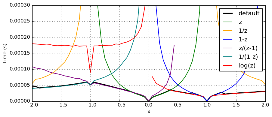
The following plot shows the time to compute $\operatorname{Li}_2(x)$ at 333-bit precision using the $\log(z)$ series and the hypergeometric series with the transformations $z$, $1/z$, $1-z$, $z/(z-1)$, $1/(1-z)$. The time for the default method which attempts to select the best algorithm automatically is shown in black.
Miscellaneous
Finally:
- Many short functions (for example: arb_one, arb_set_ui, ...) have been changed from inline functions to ordinary functions. This reduced the size of libarb.so from 23 MB to just 15 MB on my machine. Macro benchmarks suggest that there should be no slowdown, and in fact some code may speed up due to cache and branch prediction effects. Compiling the library is also slightly faster.
- New convenience functions include arb_poly_log1p_series, acb_poly_log1p_series and acb_poly_exp_pi_i_series which compute $\log(1+x)$ and $e^{\pi i x}$ of power series. The log functions compute the constant term accurately when $x \approx 0$, and the modified exponential function is useful when $x$ is an integer or half-integer (or close), just like acb_poly_sin_pi_series and related methods.
fredrikj.net |
Blog index |
 RSS feed |
Follow me on Mastodon |
Become a sponsor
RSS feed |
Follow me on Mastodon |
Become a sponsor